EECS 224: Large Language Models
This is a new course of UC Merced starting at Spring 2025. In this course, students will learn the fundamentals about the modeling, theory, ethics, and systems aspects of large language models, as well as gain hands-on experience working with them.
The Goal of This Course
Offering useful, fundemental, detailed LLM knowledge to students.
Coursework
- In-Course Question Answering
- Final Projects
In-Course Question Answering
In each class, students will be asked several questions. Each student can only answer each question one time. The student who correctly answers a question for the first time and explain the answer clearly to all the classmates will be granted 1 credit. The final scores will be calculated based on the accumulated credits throughout the whole semester. This score does not contribute to the final grading. In the final course, the students who get high scores in question answering will be highlighted as a reputation.
Final Projects
Every student should complete a final project related to LLMs and present it in the final classes. A project report should be completed before the presentation and submitted to Final Project Google Form The file should be named as “Your Name.pdf” The format should follow the 2025 ACL long paper template. Good examples are at Project Report Examples
The final project scores will be calculated through 70% Instructor’s rating + 30% Classmates’ rating. After all the presentations, every student will be asked to choose 3 best projects. The classmates’ ratings will be based on the ratings of all the classmates.
Useful Links
Lecture 1: Overview of LLMs
What is Language?
Language is a systematic means of communicating ideas or feelings using conventionalized signs, sounds, gestures, or marks.

More than 7,000 languages are spoken around the world today, shaping how we describe and perceive the world around us. Source: https://www.snexplores.org/article/lets-learn-about-the-science-of-language
Text in Language
Text represents the written form of language, converting speech and meaning into visual symbols. Key aspects include:
Basic Units of Text
Text can be broken down into hierarchical units:
- Characters: The smallest meaningful units in writing systems
- Words: Combinations of characters that carry meaning
- Sentences: Groups of words expressing complete thoughts
- Paragraphs: Collections of related sentences
- Documents: Complete texts serving a specific purpose
Text Properties
Text demonstrates several key properties:
- Linearity: Written symbols appear in sequence
- Discreteness: Clear boundaries between units
- Conventionality: Agreed-upon meanings within a language community
- Structure: Follows grammatical and syntactic rules
- Context: Meaning often depends on surrounding text
Question 1: Could you give some examples in English that a word has two different meanings across two sentences?
Based on the above properties shared by different langauges, the NLP researchers develop a unified Machine Learning technique to model language data – Large Language Models. Let’s start to learn this unfied language modeling technique.
What is a Language Model?
Mathematical Definition
A language model is fundamentally a probability distribution over sequences of words or tokens. Mathematically, it can be expressed as:
\[P(w_1, w_2, ..., w_n) = \prod_i P(w_i|w_1, ..., w_{i-1})\]where:
- \(w_1, w_2, ..., w_n\) represents a sequence of words or tokens
-
The conditional probability of word \(w_i\) given all previous words is:
\[P(w_i|w_1, ..., w_{i-1})\]
For practical implementation, this often takes the form:
\[P(w_t|context) = \text{softmax}(h(context) \cdot W)\]where:
- Target word: \(w_t\)
- Context encoding function: \(h(context)\)
- Weight matrix: \(W\)
- softmax normalizes the output into probabilities
Example 1: Sentence Probability Calculation
Consider the sentence: “I love chocolate.”
The language model predicts the following probabilities:
- \[P(\text{'I'}) = 0.2\]
- \[P(\text{'love'}|\text{'I'}) = 0.4\]
- \[P(\text{'chocolate'}|\text{'I love'}) = 0.5\]
The total probability of the sentence is calculated as:
\(P(\text{'I love chocolate'}) = P(\text{'I'}) \cdot P(\text{'love'}|\text{'I'}) \cdot P(\text{'chocolate'}|\text{'I love'})\)
\(P(\text{'I love chocolate'}) = 0.2 \cdot 0.4 \cdot 0.5 = 0.04\)
Thus, the probability of the sentence “I love chocolate” is 0.04.
Example 2: Dialogue Probability Calculation
For the dialogue:
A: “Hello, how are you?”
B: “I’m fine, thank you.”
The model provides the following probabilities:
- Speaker A’s Sentence:
- \[P(\text{'Hello'}) = 0.3\]
- \[P(\text{','}|\text{'Hello'}) = 0.8\]
- \[P(\text{'how'}|\text{'Hello ,'}) = 0.5\]
- \[P(\text{'are'}|\text{'Hello , how'}) = 0.6\]
- \[P(\text{'you'}|\text{'Hello , how are'}) = 0.7\]
- Speaker B’s Sentence:
- \[P(\text{'I'}) = 0.4\]
- \[P(\text{'m'}|\text{'I'}) = 0.5\]
- \[P(\text{'fine'}|\text{'I m'}) = 0.6\]
- \[P(\text{','}|\text{'I m fine'}) = 0.7\]
- \[P(\text{'thank'}|\text{'I m fine ,'}) = 0.8\]
- \[P(\text{'you'}|\text{'I m fine , thank'}) = 0.9\]
- Total Probability for the Dialogue:
Combine the probabilities for both sentences:
\(P(\text{'Hello, how are you? I\'m fine, thank you.'}) = P(\text{'Hello, how are you?'}) \cdot P(\text{'I\'m fine, thank you.'})\)
\(P(\text{'Hello, how are you? I\'m fine, thank you.'}) = 0.0504 \cdot 0.06048 = 0.003048192\)
Thus, the total probability of the dialogue is approximately 0.00305.
Example 3: Partial Sentence Generation
Consider the sentence: “The dog barked loudly.”
The probabilities assigned by the language model are:
- \[P(\text{'The'}) = 0.25\]
- \[P(\text{'dog'}|\text{'The'}) = 0.4\]
- \[P(\text{'barked'}|\text{'The dog'}) = 0.5\]
- \[P(\text{'loudly'}|\text{'The dog barked'}) = 0.6\]
Question 2: Calculate the total probability of the sentence \(P(\text{'The dog barked loudly'})\) using the given probabilities.
The Transformer Model: Revolutionizing Language Models
The emergence of the Transformer architecture marked a paradigm shift in how machines process and understand human language. Unlike its predecessors, which struggled with long-range patterns in text, this groundbreaking architecture introduced mechanisms that revolutionized natural language processing (NLP).
The Building Blocks of Language Understanding
From Text to Machine-Readable Format
Before any sophisticated processing can occur, raw text must be converted into a format that machines can process. This happens in two crucial stages:
- Text Segmentation
The first challenge is breaking down text into meaningful units. Imagine building with LEGO blocks - just as you need individual blocks to create complex structures, language models need discrete pieces of text to work with. These pieces, called tokens, might be:
- Complete words
- Parts of words
- Individual characters
- Special symbols
For instance, the phrase “artificial intelligence” might become [“art”, “ificial”, “intel”, “ligence”], allowing the model to recognize patterns even in unfamiliar words.
- Numerical Representation Once we have our text pieces, each token gets transformed into a numerical vector - essentially a long list of numbers. Think of this as giving each word or piece its own unique mathematical “fingerprint” that captures its meaning and relationships with other words.
Adding Sequential Understanding
One of the most innovative aspects of Transformers is how they handle word order. Rather than treating text like a bag of unrelated words, the architecture adds precise positional information to each token’s representation.
Consider how the meaning changes in these sentences:
- “The cat chased the mouse”
- “The mouse chased the cat”
The words are identical, but their positions completely change the meaning. The Transformer’s positional encoding system ensures this crucial information isn’t lost.
The Heart of the System: Information Processing
Context Through Self-Attention
The true magic of Transformers lies in their attention mechanism. Unlike humans who must read text sequentially, Transformers can simultaneously analyze relationships between all words in a text. This is similar to how you might solve a complex puzzle:
- First, you look at all the pieces simultaneously
- Then, you identify which pieces are most likely to connect
- Finally, you use these relationships to build the complete picture
In language, this means the model can:
- Resolve pronouns (“She picked up her book” - who is “her” referring to?)
- Understand idiomatic expressions (“kicked the bucket” means something very different from “kicked the ball”)
- Grasp long-distance dependencies (“The keys, which I thought I had left on the kitchen counter yesterday morning, were actually in my coat pocket”)
Real-World Applications and Impact
The Transformer architecture has enabled breakthrough applications in:
- Cross-Language Communication
- Real-time translation systems
- Multilingual document processing
- Content Creation and Analysis
- Automated report generation
- Text summarization
- Content recommendations
- Specialized Industry Applications
- Legal document analysis
- Medical record processing
- Scientific literature review
The Road Ahead
As this architecture continues to evolve, we’re seeing:
- More efficient processing methods
- Better handling of specialized domains
- Improved understanding of contextual nuances
- Enhanced ability to work with multimodal inputs
The Transformer architecture represents more than just a technical advancement - it’s a fundamental shift in how machines can understand and process human language. Its impact continues to grow as researchers and developers find new ways to apply and improve upon its core principles.
The true power of Transformers lies not just in their technical capabilities, but in how they’ve opened new possibilities for human-machine interaction and understanding. As we continue to refine and build upon this architecture, we’re moving closer to systems that can truly understand and engage with human language in all its complexity and nuance.
What are large language models?
Large language models are transformers with billions to trillions of parameters, trained on massive amounts of text data. These models have several distinguishing characteristics:
- Scale: Models contain billions of parameters and are trained on hundreds of billions of tokens
- Architecture: Based on the Transformer architecture with self-attention mechanisms
- Emergent abilities: Complex capabilities that emerge with scale
- Few-shot learning: Ability to adapt to new tasks with few examples
-
Definition: Large Language Models are artificial intelligence systems trained on vast amounts of text data, containing hundreds of billions of parameters. Unlike traditional AI models, they can understand and generate human-like text across a wide range of tasks and domains.
- Scale and Architecture:
- Typically contain >1B parameters (Some exceed 500B)
- Built on Transformer architecture with attention mechanisms
- Require massive computational resources for training
- Examples: GPT-3 (175B), PaLM (540B), LLaMA (65B)
- Key Capabilities:
- Natural language understanding and generation
- Task adaptation without fine-tuning
- Complex reasoning and problem solving
- Knowledge storage and retrieval
- Multi-turn conversation
Historical Evolution
1. Statistical Language Models (SLM) - 1990s
- Core Technology: Used statistical methods to predict next words based on previous context
- Key Features:
- N-gram models (bigram, trigram)
- Markov assumption for word prediction
- Used in early IR and NLP applications
- Limitations:
- Curse of dimensionality
- Data sparsity issues
- Limited context window
- Required smoothing techniques
2. Neural Language Models (NLM) - 2013
- Core Technology: Neural networks for language modeling
- Key Advances:
- Distributed word representations
- Multi-layer perceptron and RNN architectures
- End-to-end learning
- Better feature extraction
- Impact:
- Word2vec and similar embedding models
- Improved generalization
- Reduced need for feature engineering
3. Pre-trained Language Models (PLM) - 2018
- Core Technology: Transformer-based models with pre-training
- Key Innovations:
- BERT and bidirectional context modeling
- GPT and autoregressive modeling
- Transfer learning approach
- Fine-tuning paradigm
- Benefits:
- Context-aware representations
- Better task performance
- Reduced need for task-specific data
- More efficient training
4. Large Language Models (LLM) - 2020+
- Core Technology: Scaled-up Transformer models
- Major Breakthroughs:
- Emergence of new abilities with scale
- Few-shot and zero-shot learning
- General-purpose problem solving
- Human-like interaction capabilities
- Key Examples:
- GPT-3: First demonstration of powerful in-context learning
- ChatGPT: Advanced conversational abilities
- GPT-4: Multimodal capabilities and improved reasoning
- PaLM: Enhanced multilingual and reasoning capabilities
Key Features of LLMs
Scaling Laws
- KM Scaling Law (OpenAI):
- Describes relationship between model performance (measured by cross entropy loss $L$) and three factors:
- Model size ($N$)
- Dataset size ($D$)
- Computing power ($C$)
- Mathematical formulations:
- $L(N) = \left(\frac{N_c}{N}\right)^{\alpha_N}$, where $\alpha_N \sim 0.076$, $N_c \sim 8.8 \times 10^{13}$
- $L(D) = \left(\frac{D_c}{D}\right)^{\alpha_D}$, where $\alpha_D \sim 0.095$, $D_c \sim 5.4 \times 10^{13}$
- $L(C) = \left(\frac{C_c}{C}\right)^{\alpha_C}$, where $\alpha_C \sim 0.050$, $C_c \sim 3.1 \times 10^8$
- Predicts diminishing returns as model/data/compute scale increases
- Helps optimize resource allocation for training
- Describes relationship between model performance (measured by cross entropy loss $L$) and three factors:
- Chinchilla Scaling Law (DeepMind):
- Mathematical formulation:
- $L(N,D) = E + \frac{A}{N^\alpha} + \frac{B}{D^\beta}$
- where $E = 1.69$, $A = 406.4$, $B = 410.7$, $\alpha = 0.34$, $\beta = 0.28$
- Optimal compute allocation:
- $N_{opt}(C) = G\left(\frac{C}{6}\right)^a$
- $D_{opt}(C) = G^{-1}\left(\frac{C}{6}\right)^b$
- where $a = \frac{\alpha}{\alpha+\beta}$, $b = \frac{\beta}{\alpha+\beta}$
- Suggests equal scaling of model and data size
- More efficient compute utilization than KM scaling law
- Demonstrated superior performance with smaller models trained on more data
- Mathematical formulation:
Emergent Abilities
- In-context Learning
- Definition: Ability to learn from examples in the prompt
- Characteristics:
- No parameter updates required
- Few-shot and zero-shot capabilities
- Task adaptation through demonstrations
- Emergence Point:
- GPT-3 showed first strong results
Question 3: Design a few-shot prompt that can classify the film topic by the film name. It must be able to correctly classify more than 5 films proposed by other students. Using ChatGPT as the test LLM.
- Instruction Following
- Definition: Ability to understand and execute natural language instructions
- Requirements:
- Instruction tuning
- Multi-task training
- Natural language task descriptions
- Step-by-step Reasoning
- Definition: Ability to break down complex problems
- Techniques:
- Chain-of-thought prompting
- Self-consistency methods
- Intermediate step generation
- Benefits:
- Better problem solving
- More reliable answers
- Transparent reasoning process
Technical Elements
Architecture
- Transformer Base
- Components:
- Multi-head attention mechanism
- Feed-forward neural networks
- Layer normalization
- Positional encoding
- Variations:
- Decoder-only (GPT-style)
- Encoder-decoder (T5-style)
- Modifications for efficiency
- Components:
- Scaling Considerations
- Hardware Requirements:
- Distributed training systems
- Memory optimization
- Parallel processing
- Architecture Choices:
- Layer count
- Hidden dimension size
- Attention head configuration
- Hardware Requirements:
Training Process
- Pre-training
- Data Preparation:
- Web text
- Books
- Code
- Scientific papers
- Objectives:
- Next token prediction
- Masked language modeling
- Multiple auxiliary tasks
- Data Preparation:
- Adaptation Methods
- Instruction Tuning:
- Natural language task descriptions
- Multi-task learning
- Task generalization
- RLHF:
- Human preference learning
- Safety alignment
- Behavior optimization
- Instruction Tuning:
Utilization Techniques
- Prompting Strategies
- Basic Prompting:
- Direct instructions
- Few-shot examples
- Zero-shot prompts
- Advanced Methods:
- Chain-of-thought
- Self-consistency
- Tool augmentation
- Basic Prompting:
- Application Patterns
- Task Types:
- Generation
- Classification
- Question answering
- Coding
- Integration Methods:
- API endpoints
- Model serving
- Application backends
- Task Types:
Major Milestones
ChatGPT (2022)
- Technical Achievements
- Advanced dialogue capabilities
- Robust safety measures
- Consistent persona
- Tool integration
- Impact
- Widespread adoption
- New application paradigms
- Industry transformation
- Public AI awareness
GPT-4 (2023)
- Key Advances
- Multimodal understanding
- Enhanced reliability
- Better reasoning
- Improved safety
- Technical Features
- Predictable scaling
- Vision capabilities
- Longer context window
- Advanced system prompting
Challenges and Future Directions
Current Challenges
- Computational Resources
- Training Costs:
- Massive energy requirements
- Expensive hardware needs
- Limited accessibility
- Infrastructure Needs:
- Specialized facilities
- Cooling systems
- Power management
- Training Costs:
- Data Requirements
- Quality Issues:
- Data cleaning
- Content filtering
- Bias mitigation
- Privacy Concerns:
- Personal information
- Copyright issues
- Regulatory compliance
- Quality Issues:
- Safety and Alignment
- Technical Challenges:
- Hallucination prevention
- Truthfulness
- Bias detection
- Ethical Considerations:
- Harm prevention
- Fairness
- Transparency
- Technical Challenges:
Future Directions
- Improved Efficiency
- Architecture Innovation:
- Sparse attention
- Parameter efficiency
- Memory optimization
- Training Methods:
- Better scaling laws
- Efficient fine-tuning
- Reduced compute needs
- Architecture Innovation:
- Enhanced Capabilities
- Multimodal Understanding:
- Vision-language integration
- Audio processing
- Sensor data interpretation
- Reasoning Abilities:
- Logical deduction
- Mathematical problem solving
- Scientific reasoning
- Multimodal Understanding:
- Safety Development
- Alignment Techniques:
- Value learning
- Preference optimization
- Safety bounds
- Evaluation Methods:
- Robustness testing
- Safety metrics
- Bias assessment
- Alignment Techniques:
Summary
- LLMs represent a fundamental shift in AI capabilities
- Scale and architecture drive emergent abilities
- Continuing rapid development in capabilities
- Balance between advancement and safety
- Growing impact on society and technology
- Need for responsible development and deployment
References and Further Reading
- Scaling Laws Papers
- Emergent Abilities Research
- Safety and Alignment Studies
- Technical Documentation
- Industry Reports
Paper Reading: A Survey of Large Language Models
Lecture 2: Understanding Tokenization in Language Models
Tokenization is a fundamental concept in Natural Language Processing (NLP) that involves breaking down text into smaller units called tokens. These tokens can be words, subwords, or characters, depending on the tokenization strategy used. The choice of tokenization method can significantly impact a model’s performance and its ability to handle various languages and vocabularies.
Common Tokenization Approaches
- Word-based Tokenization
- Splits text at word boundaries (usually spaces and punctuation)
- Simple and intuitive but struggles with out-of-vocabulary words
- Requires a large vocabulary to cover most words
- Examples: Early versions of BERT used WordPiece tokenization
- Character-based Tokenization
- Splits text into individual characters
- Very small vocabulary size
- Can handle any word but loses word-level meaning
- Typically results in longer sequences
- Subword Tokenization
- Breaks words into meaningful subunits
- Balances vocabulary size and semantic meaning
- Better handles rare words
- Popular methods include:
- Byte-Pair Encoding (BPE)
- WordPiece
- Unigram
- SentencePiece
Let’s dive deep into one of the most widely used subword tokenization methods: Byte-Pair Encoding (BPE).
Byte-Pair Encoding (BPE) Tokenization
Reference Tutorial: Byte-Pair Encoding tokenization
Byte-Pair Encoding (BPE) was initially developed as an algorithm to compress texts, and then used by OpenAI for tokenization when pretraining the GPT model. It’s used by many Transformer models, including GPT, GPT-2, Llama1, Llama2, Llama3, RoBERTa, BART, and DeBERTa.
Training Algorithm
BPE training starts by computing the unique set of words used in the corpus (after the normalization and pre-tokenization steps are completed), then building the vocabulary by taking all the symbols used to write those words. As a very simple example, let’s say our corpus uses these five words:
"hug", "pug", "pun", "bun", "hugs"
The base vocabulary will then be ["b", "g", "h", "n", "p", "s", "u"]. For real-world cases, that base vocabulary will contain all the ASCII characters, at the very least, and probably some Unicode characters as well. If an example you are tokenizing uses a character that is not in the training corpus, that character will be converted to the unknown token. That’s one reason why lots of NLP models are very bad at analyzing content with emojis.
The GPT-2 and RoBERTa tokenizers (which are pretty similar) have a clever way to deal with this: they don’t look at words as being written with Unicode characters, but with bytes. This way the base vocabulary has a small size (256), but every character you can think of will still be included and not end up being converted to the unknown token. This trick is called byte-level BPE.
After getting this base vocabulary, we add new tokens until the desired vocabulary size is reached by learning merges, which are rules to merge two elements of the existing vocabulary together into a new one. So, at the beginning these merges will create tokens with two characters, and then, as training progresses, longer subwords.
At any step during the tokenizer training, the BPE algorithm will search for the most frequent pair of existing tokens (by “pair,” here we mean two consecutive tokens in a word). That most frequent pair is the one that will be merged, and we rinse and repeat for the next step.
Going back to our previous example, let’s assume the words had the following frequencies:
("hug", 10), ("pug", 5), ("pun", 12), ("bun", 4), ("hugs", 5)
meaning “hug” was present 10 times in the corpus, “pug” 5 times, “pun” 12 times, “bun” 4 times, and “hugs” 5 times. We start the training by splitting each word into characters (the ones that form our initial vocabulary) so we can see each word as a list of tokens:
("h" "u" "g", 10), ("p" "u" "g", 5), ("p" "u" "n", 12), ("b" "u" "n", 4), ("h" "u" "g" "s", 5)
Then we look at pairs. The pair (“h”, “u”) is present in the words “hug” and “hugs”, so 15 times total in the corpus. It’s not the most frequent pair, though: that honor belongs to (“u”, “g”), which is present in “hug”, “pug”, and “hugs”, for a grand total of 20 times in the vocabulary.
Thus, the first merge rule learned by the tokenizer is (“u”, “g”) -> “ug”, which means that “ug” will be added to the vocabulary, and the pair should be merged in all the words of the corpus. At the end of this stage, the vocabulary and corpus look like this:
Vocabulary: ["b", "g", "h", "n", "p", "s", "u", "ug"]
Corpus: ("h" "ug", 10), ("p" "ug", 5), ("p" "u" "n", 12), ("b" "u" "n", 4), ("h" "ug" "s", 5)
Now we have some pairs that result in a token longer than two characters: the pair (“h”, “ug”), for instance (present 15 times in the corpus). The most frequent pair at this stage is (“u”, “n”), however, present 16 times in the corpus, so the second merge rule learned is (“u”, “n”) -> “un”. Adding that to the vocabulary and merging all existing occurrences leads us to:
Vocabulary: ["b", "g", "h", "n", "p", "s", "u", "ug", "un"]
Corpus: ("h" "ug", 10), ("p" "ug", 5), ("p" "un", 12), ("b" "un", 4), ("h" "ug" "s", 5)
Now the most frequent pair is (“h”, “ug”), so we learn the merge rule (“h”, “ug”) -> “hug”, which gives us our first three-letter token. After the merge, the corpus looks like this:
Vocabulary: ["b", "g", "h", "n", "p", "s", "u", "ug", "un", "hug"]
Corpus: ("hug", 10), ("p" "ug", 5), ("p" "un", 12), ("b" "un", 4), ("hug" "s", 5)
And we continue like this until we reach the desired vocabulary size.
Tokenization Inference
Tokenization inference follows the training process closely, in the sense that new inputs are tokenized by applying the following steps:
- Splitting the words into individual characters
- Applying the merge rules learned in order on those splits
Let’s take the example we used during training, with the three merge rules learned:
("u", "g") -> "ug"
("u", "n") -> "un"
("h", "ug") -> "hug"
The word “bug” will be tokenized as ["b", "ug"]. “mug”, however, will be tokenized as ["[UNK]", "ug"] since the letter “m” was not in the base vocabulary. Likewise, the word “thug” will be tokenized as ["[UNK]", "hug"]: the letter “t” is not in the base vocabulary, and applying the merge rules results first in “u” and “g” being merged and then “h” and “ug” being merged.
Implementing BPE
Now let’s take a look at an implementation of the BPE algorithm. This won’t be an optimized version you can actually use on a big corpus; we just want to show you the code so you can understand the algorithm a little bit better.
I present the colab link for you to reproduce this part’s experiments easily: Colab BPE
Training BPE
First we need a corpus, so let’s create a simple one with a few sentences:
corpus = [
    "This is the Hugging Face Course.",
    "This chapter is about tokenization.",
    "This section shows several tokenizer algorithms.",
    "Hopefully, you will be able to understand how they are trained and generate tokens."
]
Next, we need to pre-tokenize that corpus into words. Since we are replicating a BPE tokenizer (like GPT-2), we will use the gpt2 tokenizer for the pre-tokenization:
from transformers import AutoTokenizer

# init pre tokenize function
gpt2_tokenizer = AutoTokenizer.from_pretrained("gpt2")
pre_tokenize_function = gpt2_tokenizer.backend_tokenizer.pre_tokenizer.pre_tokenize_str

# pre tokenize
pre_tokenized_corpus = [pre_tokenize_function(text) for text in corpus]
We have the output
[
    [('This', (0, 4)), ('Ġis', (4, 7)), ('Ġthe', (7, 11)), ('ĠHugging', (11, 19)), ('ĠFace', (19, 24)), ('ĠCourse', (24, 31)), ('.', (31, 32))],
    [('This', (0, 4)), ('Ġchapter', (4, 12)), ('Ġis', (12, 15)), ('Ġabout', (15, 21)), ('Ġtokenization', (21, 34)), ('.', (34, 35))],
    [('This', (0, 4)), ('Ġsection', (4, 12)), ('Ġshows', (12, 18)), ('Ġseveral', (18, 26)), ('Ġtokenizer', (26, 36)), ('Ġalgorithms', (36, 47)), ('.', (47, 48))],
    [('Hopefully', (0, 9)), (',', (9, 10)), ('Ġyou', (10, 14)), ('Ġwill', (14, 19)), ('Ġbe', (19, 22)), ('Ġable', (22, 27)), ('Ġto', (27, 30)), ('Ġunderstand', (30, 41)), ('Ġhow', (41, 45)), ('Ġthey', (45, 50)), ('Ġare', (50, 54)), ('Ġtrained', (54, 62)), ('Ġand', (62, 66)), ('Ġgenerate', (66, 75)), ('Ġtokens', (75, 82)), ('.', (82, 83))]
]
Then we compute the frequencies of each word in the corpus as we do the pre-tokenization:
from collections import defaultdict
word2count = defaultdict(int)
for split_text in pre_tokenized_corpus:
    for word, _ in split_text:
        word2count[word] += 1
The obtained word2count is as follows:
defaultdict(<class 'int'>, {'This': 3, 'Ġis': 2, 'Ġthe': 1, 'ĠHugging': 1, 'ĠFace': 1, 'ĠCourse': 1, '.': 4, 'Ġchapter': 1, 'Ġabout': 1, 'Ġtokenization': 1, 'Ġsection': 1, 'Ġshows': 1, 'Ġseveral': 1, 'Ġtokenizer': 1, 'Ġalgorithms': 1, 'Hopefully': 1, ',': 1, 'Ġyou': 1, 'Ġwill': 1, 'Ġbe': 1, 'Ġable': 1, 'Ġto': 1, 'Ġunderstand': 1, 'Ġhow': 1, 'Ġthey': 1, 'Ġare': 1, 'Ġtrained': 1, 'Ġand': 1, 'Ġgenerate': 1, 'Ġtokens': 1})
The next step is to compute the base vocabulary, formed by all the characters used in the corpus:
vocab_set = set()
for word in word2count:
    vocab_set.update(list(word))
vocabs = list(vocab_set)
The obtained base vocabulary is as follows:
['i', 't', 'p', 'o', 'r', 'm', 'e', ',', 'y', 'v', 'Ġ', 'F', 'a', 'C', 'H', '.', 'f', 'l', 'u', 'c', 'T', 'k', 'h', 'z', 'd', 'g', 'w', 'n', 's', 'b']
We now need to split each word into individual characters, to be able to start training:
word2splits = {word: [c for c in word] for word in word2count}
The output is:
'This': ['T', 'h', 'i', 's'],
'Ġis': ['Ġ', 'i', 's'],
'Ġthe': ['Ġ', 't', 'h', 'e'],
...
'Ġand': ['Ġ', 'a', 'n', 'd'],
'Ġgenerate': ['Ġ', 'g', 'e', 'n', 'e', 'r', 'a', 't', 'e'],
'Ġtokens': ['Ġ', 't', 'o', 'k', 'e', 'n', 's']
Now that we are ready for training, let’s write a function that computes the frequency of each pair. We’ll need to use this at each step of the training:
def _compute_pair2score(word2splits, word2count):
    pair2count = defaultdict(int)
    for word, word_count in word2count.items():
        split = word2splits[word]
        if len(split) == 1:
            continue
        for i in range(len(split) - 1):
            pair = (split[i], split[i + 1])
            pair2count[pair] += word_count
    return pair2count
The output is
defaultdict(<class 'int'>, {('T', 'h'): 3, ('h', 'i'): 3, ('i', 's'): 5, ('Ġ', 'i'): 2, ('Ġ', 't'): 7, ('t', 'h'): 3, ..., ('n', 's'): 1})
Now, finding the most frequent pair only takes a quick loop:
def _compute_most_score_pair(pair2count):
    best_pair = None
    max_freq = None
    for pair, freq in pair2count.items():
        if max_freq is None or max_freq < freq:
            best_pair = pair
            max_freq = freq
    return best_pair
After counting, the current pair with the highest frequency is: (‘Ġ’, ‘t’), occurring 7 times. We merge (‘Ġ’, ‘t’) into a single token and add it to the vocabulary. Simultaneously, we add the merge rule (‘Ġ’, ‘t’) to our list of merge rules.
merge_rules = []
best_pair = compute_most_score_pair(pair2score)
vocabs.append(best_pair[0] + best_pair[1])
merge_rules.append(best_pair)
Now the vocabulary is
['i', 't', 'p', 'o', 'r', 'm', 'e', ',', 'y', 'v', 'Ġ', 'F', 'a', 'C', 'H', '.', 'f', 'l', 'u', 'c', 'T', 'k', 'h', 'z', 'd', 'g', 'w', 'n', 's', 'b',
'Ġt']
Based on the updated vocabulary, we re-split word2count. For implementation, we can directly apply the new merge rule (‘Ġ’, ‘t’) to the existing word2split. This is more efficient than performing a complete re-split, as we only need to apply the latest merge rule to the existing splits.
def _merge_pair(a, b, word2splits):
    new_word2splits = dict()
    for word, split in word2splits.items():
        if len(split) == 1:
            new_word2splits[word] = split
            continue
        i = 0
        while i < len(split) - 1:
            if split[i] == a and split[i + 1] == b:
                split = split[:i] + [a + b] + split[i + 2:]
            else:
                i += 1
        new_word2splits[word] = split
    return new_word2splits
The new word2split is
{'This': ['T', 'h', 'i', 's'],
'Ġis': ['Ġ', 'i', 's'],
'Ġthe': ['Ġt', 'h', 'e'],
'ĠHugging': ['Ġ', 'H', 'u', 'g', 'g', 'i', 'n', 'g'],
...
'Ġtokens': ['Ġt', 'o', 'k', 'e', 'n', 's']}
As we can see, the new word2split now contains the newly merged token “Ġt”. We repeat this iterative process until the vocabulary size reaches our predefined target size.
while len(vocabs) < vocab_size:
    pair2score = compute_pair2score(word2splits, word2count)
    best_pair = compute_most_score_pair(pair2score)
    vocabs.append(best_pair[0] + best_pair[1])
    merge_rules.append(best_pair)
    word2splits = merge_pair(best_pair[0], best_pair[1], word2splits)
Let’s say our target vocabulary size is 50. After the above iterations, we obtain the following vocabulary and merge rules:
vocabs = ['i', 't', 'p', 'o', 'r', 'm', 'e', ',', 'y', 'v', 'Ġ', 'F', 'a', 'C', 'H', '.', 'f', 'l', 'u', 'c', 'T', 'k', 'h', 'z', 'd', 'g', 'w', 'n', 's', 'b', 'Ġt', 'is', 'er', 'Ġa', 'Ġto', 'en', 'Th', 'This', 'ou', 'se', 'Ġtok', 'Ġtoken', 'nd', 'Ġis', 'Ġth', 'Ġthe', 'in', 'Ġab', 'Ġtokeni', 'Ġtokeniz']

merge_rules = [('Ġ', 't'), ('i', 's'), ('e', 'r'), ('Ġ', 'a'), ('Ġt', 'o'), ('e', 'n'), ('T', 'h'), ('Th', 'is'), ('o', 'u'), ('s', 'e'), ('Ġto', 'k'), ('Ġtok', 'en'), ('n', 'd'), ('Ġ', 'is'), ('Ġt', 'h'), ('Ġth', 'e'), ('i', 'n'), ('Ġa', 'b'), ('Ġtoken', 'i'), ('Ġtokeni', 'z')]
Thus, we have completed the training of our BPE tokenizer based on the given corpus. This trained tokenizer, consisting of the vocabulary and merge rules, can now be used to tokenize new input text using the learned subword patterns.
BPE’s Inference
During the inference phase, given a sentence, we need to split it into a sequence of tokens. The implementation involves two main steps:
First, we pre-tokenize the sentence and split it into character-level sequences
Then, we apply the merge rules sequentially to form larger tokens
def tokenize(text):
    # pre tokenize
    words = [word for word, _ in pre_tokenize_str(text)]
    # split into char level
    splits = [[c for c in word] for word in words]
    # apply merge rules
    for merge_rule in merge_rules:
        for index, split in enumerate(splits):
            i = 0
            while i < len(split) - 1:
                if split[i] == merge_rule[0] and split[i + 1] == merge_rule[1]:
                    split = split[:i] + ["".join(merge_rule)] + split[i + 2:]
                else:
                    i += 1
            splits[index] = split
    return sum(splits, [])
For example:
>>> tokenize("This is not a token.")
>>> ['This', 'Ġis', 'Ġ', 'n', 'o', 't', 'Ġa', 'Ġtoken', '.']
Question 1: Given the tokenizer introduced in Lecture 2, what is the tokenization result of the string “This is a token.”
Lecture 3: Transformer Architecture
Table of Contents
- Introduction
- Background
- General Transformer Architecture
- Attention Mechanism
- Position-Wise Feed-Forward Networks
- Training and Optimization
- Conclusion
Introduction
The Transformer model is a powerful deep learning architecture that has achieved groundbreaking results in various fields—most notably in Natural Language Processing (NLP), computer vision, and speech recognition—since it was introduced in Attention Is All You Need (Vaswani et al., 2017). Its core component is the self-attention mechanism, which efficiently handles long-range dependencies in sequences while allowing for extensive parallelization. Many subsequent models, such as BERT, GPT, Vision Transformer (ViT), and multimodal Transformers, are built upon this foundational structure.
Background
Before the Transformer, sequential modeling primarily relied on Recurrent Neural Networks (RNNs) or Convolutional Neural Networks (CNNs). These networks often struggled with capturing long-distance dependencies, parallelization, and computational efficiency. In contrast, the self-attention mechanism of Transformers captures global dependencies across input and output sequences simultaneously and offers excellent parallelization capabilities.
General Transformer Architecture
Modern Transformer architectures typically fall into one of three categories: encoder-decoder, encoder-only, or decoder-only, depending on the application scenario.
Encoder-Decoder Transformers
An encoder-decoder Transformer first encodes the input sequence into a contextual representation, then the decoder uses this encoded information to generate the target sequence. Typical applications include machine translation and text summarization. Models like T5 and MarianMT are representative of this structure.
Encoder-Only Transformers
Encoder-only models focus on learning bidirectional contextual representations of input sequences for classification, retrieval, and language understanding tasks. BERT and its variants (RoBERTa, ALBERT, etc.) belong to this category.
Decoder-Only Transformers
Decoder-only models generate outputs in an autoregressive manner, making them well-suited for text generation, dialogue systems, code generation, and more. GPT series, LLaMA, and PaLM are examples of this type.
Attention Mechanism
The core of the Transformer lies in its attention mechanism, which allows the model to focus on the most relevant parts of the input sequence given a query. Below, we detail the Scaled Dot-Product Attention and the Multi-Head Attention mechanisms.
What is Attention?
The attention mechanism describes a recent new group of layers in neural networks that has attracted a lot of interest in the past few years, especially in sequence tasks. There are a lot of different possible definitions of “attention” in the literature, but the one we will use here is the following: the attention mechanism describes a weighted average of (sequence) elements with the weights dynamically computed based on an input query and elements’ keys. So what does this exactly mean? The goal is to take an average over the features of multiple elements. However, instead of weighting each element equally, we want to weight them depending on their actual values. In other words, we want to dynamically decide on which inputs we want to “attend” more than others. In particular, an attention mechanism has usually four parts we need to specify:
- Query: The query is a feature vector that describes what we are looking for in the sequence, i.e. what would we maybe want to pay attention to.
- Keys: For each input element, we have a key which is again a feature vector. This feature vector roughly describes what the element is “offering”, or when it might be important. The keys should be designed such that we can identify the elements we want to pay attention to based on the query.
- Values: For each input element, we also have a value vector. This feature vector is the one we want to average over.
- Score function: To rate which elements we want to pay attention to, we need to specify a score function $f_{attn}$. The score function takes the query and a key as input, and output the score/attention weight of the query-key pair. It is usually implemented by simple similarity metrics like a dot product, or a small MLP.
The weights of the average are calculated by a softmax over all score function outputs. Hence, we assign those value vectors a higher weight whose corresponding key is most similar to the query. If we try to describe it with pseudo-math, we can write:
\[\alpha_i = \frac{\exp\left(f_{attn}\left(\text{key}_i, \text{query}\right)\right)}{\sum_j \exp\left(f_{attn}\left(\text{key}_j, \text{query}\right)\right)}, \hspace{5mm} \text{out} = \sum_i \alpha_i \cdot \text{value}_i\]Visually, we can show the attention over a sequence of words as follows:

Attention Example
For every word, we have one key and one value vector. The query is compared to all keys with a score function (in this case the dot product) to determine the weights. The softmax is not visualized for simplicity. Finally, the value vectors of all words are averaged using the attention weights.
Most attention mechanisms differ in terms of what queries they use, how the key and value vectors are defined, and what score function is used. The attention applied inside the Transformer architecture is called self-attention. In self-attention, each sequence element provides a key, value, and query. For each element, we perform an attention layer where based on its query, we check the similarity of the all sequence elements’ keys, and returned a different, averaged value vector for each element. We will now go into a bit more detail by first looking at the specific implementation of the attention mechanism which is in the Transformer case the scaled dot product attention.
Scaled Dot-Product Attention
Given a query matrix $Q$, key matrix $K$, and value matrix $V$, the attention formula is:
\[\text{Attention}(Q, K, V) = \text{softmax}\Bigl( \frac{QK^T}{\sqrt{d_k}} \Bigr)V\]where $d_k$ is the dimensionality of the key vectors (often the same as the query dimensionality). Every row of $Q$ corresponds a token’s embedding.
Example 1: Detailed Numerical Computation
Suppose we have the following matrices (small dimensions chosen for illustrative purposes):
\[Q = \begin{bmatrix} 1 & 0 \\ 0 & 1 \\ 1 & 1 \end{bmatrix}, \quad K = \begin{bmatrix} 1 & 1 \\ 0 & 1 \\ 1 & 0 \end{bmatrix}, \quad V = \begin{bmatrix} 0 & 2 \\ 1 & 1 \\ 2 & 0 \end{bmatrix}\]-
Compute $QK^T$
\[QK^T = \begin{bmatrix} 1 & 0 & 1 \\ 1 & 1 & 0 \\ 2 & 1 & 1 \end{bmatrix}\]
According to the example setup: -
Scale by $\sqrt{d_k}$
\[\frac{QK^T}{\sqrt{2}} \approx \begin{bmatrix} 0.71 & 0 & 0.71 \\ 0.71 & 0.71 & 0 \\ 1.41 & 0.71 & 0.71 \end{bmatrix}\]
Here, $d_k = 2$. Thus, $\sqrt{2} \approx 1.41$. So, -
Apply softmax row-wise
The softmax of a vector $x$ is given by \(\text{softmax}(x_i) = \frac{e^{x_i}}{\sum_j e^{x_j}}.\) Let’s calculate this row by row:- Row 1: $[0.71, 0, 0.71]$
- Calculate exponentials:
- $e^{0.71} \approx 2.034$ (for the 1st and 3rd elements)
- $e^{0} = 1$ (for the 2nd element)
- Sum of exponentials: $2.034 + 1 + 2.034 \approx 5.068$
- Softmax values:
- $\frac{2.034}{5.068} \approx 0.401$
- $\frac{1}{5.068} \approx 0.197$
- $\frac{2.034}{5.068} \approx 0.401$
- Final result: $[0.401, 0.197, 0.401]$ ≈ $[0.40, 0.20, 0.40]$
- Calculate exponentials:
- Row 2: $[0.71, 0.71, 0]$
- Calculate exponentials:
- $e^{0.71} \approx 2.034$ (for the 1st and 2nd elements)
- $e^{0} = 1$ (for the 3rd element)
- Sum of exponentials: $2.034 + 2.034 + 1 \approx 5.068$
- Softmax values:
- $\frac{2.034}{5.068} \approx 0.401$
- $\frac{2.034}{5.068} \approx 0.401$
- $\frac{1}{5.068} \approx 0.197$
- Final result: $[0.401, 0.401, 0.197]$ ≈ $[0.40, 0.40, 0.20]$
- Calculate exponentials:
- Row 3: $[1.41, 0.71, 0.71]$
- Calculate exponentials:
- $e^{1.41} \approx 4.096$
- $e^{0.71} \approx 2.034$ (for the 2nd and 3rd elements)
- Sum of exponentials: $4.096 + 2.034 + 2.034 \approx 8.164$
- Softmax values:
- $\frac{4.096}{8.164} \approx 0.501$
- $\frac{2.034}{8.164} \approx 0.249$
- $\frac{2.034}{8.164} \approx 0.249$
- Final result: $[0.501, 0.249, 0.249]$ ≈ $[0.50, 0.25, 0.25]$
- Calculate exponentials:
The final softmax matrix $\alpha$ is: \(\alpha = \begin{bmatrix} 0.40 & 0.20 & 0.40 \\ 0.40 & 0.40 & 0.20 \\ 0.50 & 0.25 & 0.25 \end{bmatrix}\)
Key observations about the softmax results:
- All output values are between 0 and 1
- Each row sums to 1
- Equal input values (Row 1) result in equal output probabilities
- Larger input values receive larger output probabilities (middle values in Rows 2 and 3)
(slight rounding applied).
- Row 1: $[0.71, 0, 0.71]$
-
Multiply by (V)
\(\text{Attention}(Q, K, V) = \alpha V.\)
-
Row 1 weights ([0.40, 0.20, 0.40]) on (V):
\[0.40 \times [0,2] + 0.20 \times [1,1] + 0.40 \times [2,0] = [0 + 0.20 + 0.80,\; 0.80 + 0.20 + 0] = [1.00,\; 1.00].\] -
Row 2 weights ([0.40, 0.40, 0.20]):
\[0.40 \times [0,2] + 0.40 \times [1,1] + 0.20 \times [2,0] = [0,\;0.80] + [0.40,\;0.40] + [0.40,\;0] = [0.80,\;1.20].\] -
Row 3 weights ([0.50, 0.25, 0.25]):
\[0.50 \times [0,2] + 0.25 \times [1,1] + 0.25 \times [2,0] = [0,\;1.0] + [0.25,\;0.25] + [0.50,\;0] = [0.75,\;1.25].\]
Final Output:
\[\begin{bmatrix} 1.00 & 1.00 \\ 0.80 & 1.20 \\ 0.75 & 1.25 \end{bmatrix}\](rounded values).
-
Example 2: Another Small-Dimension Example
Let us consider an even smaller example:
\[Q = \begin{bmatrix} 1 & 1 \end{bmatrix}, \quad K = \begin{bmatrix} 1 & 0 \\ 0 & 1 \end{bmatrix}, \quad V = \begin{bmatrix} 2 & 3 \\ 4 & 1 \end{bmatrix}.\]Here, $Q$ is $1 \times 2$, $K$ is $2 \times 2$, and $V$ is $2 \times 2$.
-
Compute $QK^T$
\[QK^T = QK = \begin{bmatrix} 1 & 1 \end{bmatrix} \begin{bmatrix} 1 & 0 \\ 0 & 1 \end{bmatrix} = \begin{bmatrix} 1 & 1 \end{bmatrix}.\]
Since $K$ is a square matrix, $K^T = K$: -
Scale by $\sqrt{d_k}$
\[\frac{[1,\;1]}{1.41} \approx [0.71,\;0.71].\]
$d_k = 2$. Thus, $\frac{1}{\sqrt{2}} \approx \frac{1}{1.41} \approx 0.71$. So -
Softmax
$[0.71, 0.71]$ has equal values, so the softmax is $[0.5, 0.5]$. -
Multiply by $V$
\[[0.5,\;0.5] \begin{bmatrix} 2 & 3 \\ 4 & 1 \end{bmatrix} = 0.5 \times [2,3] + 0.5 \times [4,1] = [1,1.5] + [2,0.5] = [3,2].\]
Final Output: $[3,\;2]$.
Example 3: Larger Q and K with V as a Column Vector
Let us consider an example where $Q$ and $K$ have a larger dimension, but $V$ has only one column:
\[Q = \begin{bmatrix} 1 & 1 & 1 & 1 \end{bmatrix}, \quad K = \begin{bmatrix} 1 & 0 & 0 & 0 \\ 0 & 1 & 0 & 0 \\ 0 & 0 & 1 & 0 \\ 0 & 0 & 0 & 1 \end{bmatrix}, \quad V = \begin{bmatrix} 2 \\ 4 \\ 6 \\ 8 \end{bmatrix}.\]In-Course Question: Attention computation result of the above Q, K, V.
Multi-Head Attention
Multi-head attention projects $Q, K, V$ into multiple subspaces and performs several parallel scaled dot-product attentions (referred to as “heads”). These are concatenated, then transformed via a final linear projection:
\[\text{MultiHead}(Q, K, V) = \text{Concat}(\text{head}_1, \ldots, \text{head}_h) W^O,\]where each head is computed as:
\[\text{head}_i = \text{Attention}(Q W_i^Q, K W_i^K, V W_i^V).\]Below are multiple examples illustrating how multi-head attention calculations are performed, with increasingly detailed numeric demonstrations.
Example 1: Two-Head Attention Computation (Conceptual Illustration)
Let us assume we have a 2-head setup ($h = 2$), each head operating on half the dimension of $Q, K, V$. For instance, if the original dimension is 4, each head dimension could be 2.
-
Step 1: Linear transformations and splitting
\[Q W^Q \rightarrow [Q_1,\ Q_2], \quad K W^K \rightarrow [K_1,\ K_2], \quad V W^V \rightarrow [V_1,\ V_2].\]Here, $[Q_1,\ Q_2]$ means we split the transformed $Q$ along its last dimension into two sub-matrices (head 1 and head 2).
-
Step 2: Compute scaled dot-product attention for each head
\[\text{head}_1 = \text{Attention}(Q_1, K_1, V_1), \quad \text{head}_2 = \text{Attention}(Q_2, K_2, V_2).\]Suppose after computation:
\[\text{head}_1 = \begin{bmatrix} h_{11} & h_{12} \\ h_{21} & h_{22} \\ h_{31} & h_{32} \end{bmatrix}, \quad \text{head}_2 = \begin{bmatrix} g_{11} & g_{12} \\ g_{21} & g_{22} \\ g_{31} & g_{32} \end{bmatrix}.\] -
Step 3: Concatenate and apply final linear transform
\[\text{Concat}(\text{head}_1, \text{head}_2) = \begin{bmatrix} h_{11} & h_{12} & g_{11} & g_{12} \\ h_{21} & h_{22} & g_{21} & g_{22} \\ h_{31} & h_{32} & g_{31} & g_{32} \end{bmatrix}.\]
Concatenating the heads yields a $3 \times 4$ matrix (if each head is $3 \times 2$):We then multiply by $W^O$ (e.g., a $4 \times 4$ matrix) to get the final multi-head attention output.
Note: Actual numeric computation requires specifying all projection matrices $W_i^Q, W_i^K, W_i^V, W^O$ and the input $Q, K, V$. Below, we provide more concrete numeric examples.
Example 2: Two-Head Attention with Full Numerical Details
In this example, we will provide explicit numbers for a 2-head setup. We will assume each of $Q, K, V$ has shape $(3,4)$: there are 3 “tokens” (or time steps), each with a hidden size of 4. We split that hidden size into 2 heads, each with size 2.
Step 0: Define inputs and parameters
Let
We also define the projection matrices for the two heads. For simplicity, we assume each projection matrix has shape $(4,2)$ (since we project dimension 4 down to dimension 2), and $W^O$ will have shape $(4,4)$ to map the concatenated result $(3,4)$ back to $(3,4)$.
Let’s define:
\[W^Q_1 = \begin{bmatrix} 1 & 0\\ 0 & 1\\ 1 & 0\\ 0 & 1 \end{bmatrix}, \quad W^K_1 = \begin{bmatrix} 1 & 0\\ 0 & 1\\ 0 & 1\\ 1 & 0 \end{bmatrix}, \quad W^V_1 = \begin{bmatrix} 1 & 0\\ 0 & 1\\ 1 & 0\\ 0 & 1 \end{bmatrix},\] \[W^Q_2 = \begin{bmatrix} 0 & 1\\ 1 & 0\\ 1 & 1\\ 0 & 0 \end{bmatrix}, \quad W^K_2 = \begin{bmatrix} 0 & 1\\ 1 & 0\\ 1 & 0\\ 1 & 1 \end{bmatrix}, \quad W^V_2 = \begin{bmatrix} 0 & 1\\ 1 & 1\\ 0 & 1\\ 1 & 0 \end{bmatrix}.\]And let:
\[W^O = \begin{bmatrix} 1 & 0 & 0 & 1\\ 0 & 1 & 1 & 0\\ 1 & 0 & 1 & 0\\ 0 & 1 & 0 & 1 \end{bmatrix}.\]We will go step by step.
Step 1: Compute $Q_1, K_1, V_1$ for Head 1
\[Q_1 = Q \times W^Q_1,\quad K_1 = K \times W^K_1,\quad V_1 = V \times W^V_1.\]-
$Q_1 = Q W^Q_1$.
\[Q = \begin{bmatrix} 1 & 2 & 1 & 0\\ 0 & 1 & 1 & 1\\ 1 & 0 & 2 & 1 \end{bmatrix}, \quad W^Q_1 = \begin{bmatrix} 1 & 0\\ 0 & 1\\ 1 & 0\\ 0 & 1 \end{bmatrix}.\]
Each row of $Q$ is multiplied by $W^Q_1$:-
Row 1 of $Q$: $[1,2,1,0]$
\[[1,2,1,0] \begin{bmatrix} 1 & 0\\ 0 & 1\\ 1 & 0\\ 0 & 1 \end{bmatrix} = [1*1 + 2*0 + 1*1 + 0*0,\; 1*0 + 2*1 + 1*0 + 0*1] = [2,\;2].\] -
Row 2: $[0,1,1,1]$
\[[0,1,1,1] \begin{bmatrix} 1 & 0\\ 0 & 1\\ 1 & 0\\ 0 & 1 \end{bmatrix} = [1,\;2].\] -
Row 3: $[1,0,2,1]$
\[[1,0,2,1] \begin{bmatrix} 1 & 0\\ 0 & 1\\ 1 & 0\\ 0 & 1 \end{bmatrix} = [3,\;1].\]
Thus,
\[Q_1 = \begin{bmatrix} 2 & 2\\ 1 & 2\\ 3 & 1 \end{bmatrix}.\] -
-
$K_1 = K W^K_1$.
\[K = \begin{bmatrix} 1 & 1 & 0 & 2\\ 2 & 1 & 1 & 0\\ 0 & 1 & 1 & 1 \end{bmatrix},\quad W^K_1 = \begin{bmatrix} 1 & 0\\ 0 & 1\\ 0 & 1\\ 1 & 0 \end{bmatrix}.\]-
Row 1: $[1,1,0,2]$
\[[1,1,0,2] \times \begin{bmatrix} 1 & 0\\ 0 & 1\\ 0 & 1\\ 1 & 0 \end{bmatrix} = [3,\;1].\] -
Row 2: $[2,1,1,0]$
\[[2,1,1,0] \times \begin{bmatrix} 1 & 0\\ 0 & 1\\ 0 & 1\\ 1 & 0 \end{bmatrix} = [2,\;2].\] -
Row 3: $[0,1,1,1]$
\[[0,1,1,1] \times \begin{bmatrix} 1 & 0\\ 0 & 1\\ 0 & 1\\ 1 & 0 \end{bmatrix} = [1,\;2].\]
So,
\[K_1 = \begin{bmatrix} 3 & 1\\ 2 & 2\\ 1 & 2 \end{bmatrix}.\] -
-
$V_1 = V W^V_1$.
\[V = \begin{bmatrix} 1 & 1 & 0 & 0\\ 0 & 2 & 1 & 1\\ 1 & 1 & 2 & 2 \end{bmatrix},\quad W^V_1 = \begin{bmatrix} 1 & 0\\ 0 & 1\\ 1 & 0\\ 0 & 1 \end{bmatrix}.\]-
Row 1: $[1,1,0,0]$
\[[1,1,0,0] \times \begin{bmatrix} 1 & 0\\ 0 & 1\\ 1 & 0\\ 0 & 1 \end{bmatrix} = [1,\;1].\] -
Row 2: $[0,2,1,1]$
\[[0,2,1,1] \times \begin{bmatrix} 1 & 0\\ 0 & 1\\ 1 & 0\\ 0 & 1 \end{bmatrix} = [1,\;3].\] -
Row 3: $[1,1,2,2]$
\[[1,1,2,2] \times \begin{bmatrix} 1 & 0\\ 0 & 1\\ 1 & 0\\ 0 & 1 \end{bmatrix} = [3,\;3].\]
Therefore,
\[V_1 = \begin{bmatrix} 1 & 1\\ 1 & 3\\ 3 & 3 \end{bmatrix}.\] -
Step 2: Compute $Q_2, K_2, V_2$ for Head 2
\[Q_2 = Q \times W^Q_2,\quad K_2 = K \times W^K_2,\quad V_2 = V \times W^V_2.\]-
$Q_2 = Q W^Q_2$:
\[W^Q_2 = \begin{bmatrix} 0 & 1\\ 1 & 0\\ 1 & 1\\ 0 & 0 \end{bmatrix}.\]-
Row 1 $[1,2,1,0]$:
\[[1,2,1,0] \times \begin{bmatrix} 0 & 1\\ 1 & 0\\ 1 & 1\\ 0 & 0 \end{bmatrix} = [3,\;2].\] -
Row 2 $[0,1,1,1]$:
\[[0,1,1,1] \times \begin{bmatrix} 0 & 1\\ 1 & 0\\ 1 & 1\\ 0 & 0 \end{bmatrix} = [2,\;1].\] -
Row 3 $[1,0,2,1]$:
\[[1,0,2,1] \times \begin{bmatrix} 0 & 1\\ 1 & 0\\ 1 & 1\\ 0 & 0 \end{bmatrix} = [2,\;3].\]
Hence,
\[Q_2 = \begin{bmatrix} 3 & 2\\ 2 & 1\\ 2 & 3 \end{bmatrix}.\] -
-
$K_2 = K W^K_2$:
\[W^K_2 = \begin{bmatrix} 0 & 1\\ 1 & 0\\ 1 & 0\\ 1 & 1 \end{bmatrix}.\]-
Row 1 $[1,1,0,2]$:
\[[1,1,0,2] \times \begin{bmatrix} 0 & 1\\ 1 & 0\\ 1 & 0\\ 1 & 1 \end{bmatrix} = [3,\;3].\] -
Row 2 $[2,1,1,0]$:
\[[2,1,1,0] \times \begin{bmatrix} 0 & 1\\ 1 & 0\\ 1 & 0\\ 1 & 1 \end{bmatrix} = [2,\;2].\] -
Row 3 $[0,1,1,1]$:
\[[0,1,1,1] \times \begin{bmatrix} 0 & 1\\ 1 & 0\\ 1 & 0\\ 1 & 1 \end{bmatrix} = [3,\;1].\]
So,
\[K_2 = \begin{bmatrix} 3 & 3\\ 2 & 2\\ 3 & 1 \end{bmatrix}.\] -
-
$V_2 = V W^V_2$:
\[W^V_2 = \begin{bmatrix} 0 & 1\\ 1 & 1\\ 0 & 1\\ 1 & 0 \end{bmatrix}.\]-
Row 1 $[1,1,0,0]$:
\[[1,1,0,0] \times \begin{bmatrix} 0 & 1\\ 1 & 1\\ 0 & 1\\ 1 & 0 \end{bmatrix} = [1,\;2].\] -
Row 2 $[0,2,1,1]$:
\[[0,2,1,1] \times \begin{bmatrix} 0 & 1\\ 1 & 1\\ 0 & 1\\ 1 & 0 \end{bmatrix} = [3,\;3].\] -
Row 3 $[1,1,2,2]$:
\[[1,1,2,2] \times \begin{bmatrix} 0 & 1\\ 1 & 1\\ 0 & 1\\ 1 & 0 \end{bmatrix} = [3,\;4].\]
Thus,
\[V_2 = \begin{bmatrix} 1 & 2\\ 3 & 3\\ 3 & 4 \end{bmatrix}.\] -
Step 3: Compute each head’s Scaled Dot-Product Attention
We now have for head 1:
\[Q_1 = \begin{bmatrix}2 & 2\\1 & 2\\3 & 1\end{bmatrix},\; K_1 = \begin{bmatrix}3 & 1\\2 & 2\\1 & 2\end{bmatrix},\; V_1 = \begin{bmatrix}1 & 1\\1 & 3\\3 & 3\end{bmatrix}.\]Similarly for head 2:
\[Q_2 = \begin{bmatrix}3 & 2\\2 & 1\\2 & 3\end{bmatrix},\; K_2 = \begin{bmatrix}3 & 3\\2 & 2\\3 & 1\end{bmatrix},\; V_2 = \begin{bmatrix}1 & 2\\3 & 3\\3 & 4\end{bmatrix}.\]Assume each key vector dimension is $d_k = 2$. Hence the scale is $\frac{1}{\sqrt{2}} \approx 0.707$.
- Head 1:
-
$Q_1 K_1^T$.
$K_1^T$ is
\[\begin{bmatrix} 3 & 2 & 1\\ 1 & 2 & 2 \end{bmatrix}.\] \[Q_1 K_1^T = \begin{bmatrix} 2 & 2\\ 1 & 2\\ 3 & 1 \end{bmatrix} \times \begin{bmatrix} 3 & 2 & 1\\ 1 & 2 & 2 \end{bmatrix} = \begin{bmatrix} 8 & 8 & 6\\ 5 & 6 & 5\\ 10 & 8 & 5 \end{bmatrix}.\] -
Scale: $\frac{Q_1 K_1^T}{\sqrt{2}}$:
\[\approx \begin{bmatrix} 5.66 & 5.66 & 4.24\\ 3.54 & 4.24 & 3.54\\ 7.07 & 5.66 & 3.54 \end{bmatrix}.\] -
Apply softmax row-wise (approx results after exponentiation and normalization):
\[\alpha_1 \approx \begin{bmatrix} 0.45 & 0.45 & 0.11\\ 0.25 & 0.50 & 0.25\\ 0.79 & 0.19 & 0.02 \end{bmatrix}.\] -
Multiply by $V_1$:
\[\text{head}_1 = \alpha_1 \times V_1.\]Approximating:
\[\text{head}_1 \approx \begin{bmatrix} 1.23 & 2.13\\ 1.50 & 2.50\\ 1.04 & 1.42 \end{bmatrix}.\]
-
- Head 2:
-
$Q_2 K_2^T$.
\[Q_2 = \begin{bmatrix} 3 & 2\\ 2 & 1\\ 2 & 3 \end{bmatrix},\quad K_2 = \begin{bmatrix} 3 & 3\\ 2 & 2\\ 3 & 1 \end{bmatrix}.\]Then
\[K_2^T = \begin{bmatrix} 3 & 2 & 3\\ 3 & 2 & 1 \end{bmatrix}.\] \[Q_2 K_2^T = \begin{bmatrix} 15 & 10 & 11\\ 9 & 6 & 7\\ 15 & 10 & 9 \end{bmatrix}.\] -
Scale: multiply by $1/\sqrt{2} \approx 0.707$:
\[\approx \begin{bmatrix} 10.61 & 7.07 & 7.78\\ 6.36 & 4.24 & 4.95\\ 10.61 & 7.07 & 6.36 \end{bmatrix}.\] -
Softmax row-wise (approx):
\[\alpha_2 \approx \begin{bmatrix} 0.92 & 0.03 & 0.05\\ 0.73 & 0.09 & 0.18\\ 0.96 & 0.03 & 0.01 \end{bmatrix}.\] -
Multiply by $V_2$:
\[V_2 = \begin{bmatrix} 1 & 2\\ 3 & 3\\ 3 & 4 \end{bmatrix}.\]Approximating:
\[\text{head}_2 \approx \begin{bmatrix} 1.16 & 2.13\\ 1.53 & 2.45\\ 1.09 & 2.06 \end{bmatrix}.\]
-
Step 4: Concatenate and apply $W^O$
We now concatenate $\text{head}_1$ and $\text{head}_2$ horizontally to form a $(3 \times 4)$ matrix:
Finally, multiply by $W^O$ $(4 \times 4)$:
\[\text{Output} = (\text{Concat}(\text{head}_1, \text{head}_2)) \times W^O.\]Where
\[W^O = \begin{bmatrix} 1 & 0 & 0 & 1\\ 0 & 1 & 1 & 0\\ 1 & 0 & 1 & 0\\ 0 & 1 & 0 & 1 \end{bmatrix}.\]We can do a row-by-row multiplication to get the final multi-head attention output (details omitted for brevity).
Example 3: Three-Head Attention with Another Set of Numbers (Short Demonstration)
For completeness, suppose we wanted $h=3$ heads, each of dimension $\frac{d_{\text{model}}}{3}$. The steps are exactly the same:
- Project $Q, K, V$ into three subspaces via $W^Q_i, W^K_i, W^V_i$.
- Perform scaled dot-product attention for each head:
$\text{head}_i = \text{Attention}(Q_i, K_i, V_i)$. - Concatenate all heads: $\text{Concat}(\text{head}_1, \text{head}_2, \text{head}_3)$.
- Multiply by $W^O$.
Each numeric calculation is analogous to the 2-head case—just with different shapes (e.g., each head might have dimension 4/3 if the original dimension is 4, which typically would be handled with rounding or a slightly different total dimension). The procedure remains identical in principle.
Position-Wise Feed-Forward Networks
Each layer in a Transformer includes a position-wise feed-forward network (FFN) that applies a linear transformation and activation to each position independently:
\[\text{FFN}(x) = \max(0,\; xW_1 + b_1)\, W_2 + b_2,\]where $\max(0, \cdot)$ is the ReLU activation function.
Example: Numerical Computation of the Feed-Forward Network
Let
\[x = \begin{bmatrix} 1 & 0 \\ 0 & 1 \\ 1 & 1 \end{bmatrix},\quad W_1 = \begin{bmatrix} 1 & 1 \\ 0 & 1 \end{bmatrix},\quad b_1 = \begin{bmatrix} 0 & 1 \end{bmatrix},\quad W_2 = \begin{bmatrix} 1 & 0 \\ 2 & 1 \end{bmatrix},\quad b_2 = \begin{bmatrix} 1 & -1 \end{bmatrix}.\]- Compute $xW_1 + b_1$
-
Row 1: $[1, 0]$
\[[1, 0] \begin{bmatrix} 1 & 1 \\ 0 & 1 \end{bmatrix} = [1, 1],\]then add $[0, 1]$ to get $[1, 2]$.
-
Row 2: $[0, 1]$
\[[0,1]\times \begin{bmatrix}1 & 1\\0 & 1\end{bmatrix} = [0, 1],\]plus $[0, 1]$ = $[0, 2]$.
-
Row 3: $[1,1]$
\[[1,1]\times \begin{bmatrix}1 & 1\\0 & 1\end{bmatrix} = [1, 2],\]plus $[0, 1]$ = $[1, 3]$.
So
\[X_1 = \begin{bmatrix} 1 & 2\\ 0 & 2\\ 1 & 3 \end{bmatrix}.\] -
-
ReLU activation
\[\text{ReLU}(X_1) = X_1.\]
$\max(0, X_1)$ leaves nonnegative elements unchanged. All entries are already $\ge0$, so -
Multiply by $W_2$ and add $b_2$
\[W_2 = \begin{bmatrix} 1 & 0\\ 2 & 1 \end{bmatrix},\quad b_2 = [1, -1].\] \[X_2 = X_1 W_2.\]-
Row 1 of $X_1$: $[1,2]$
\([1,2] \begin{bmatrix} 1\\2 \end{bmatrix} = 1*1 +2*2=5, \quad [1,2] \begin{bmatrix} 0\\1 \end{bmatrix} = 0 +2=2.\) So $[5,2]$.
-
Row 2: $[0,2]$
\[[0,2] \begin{bmatrix}1\\2\end{bmatrix}=4,\quad [0,2] \begin{bmatrix}0\\1\end{bmatrix}=2.\] -
Row 3: $[1,3]$
\[[1,3]\begin{bmatrix}1\\2\end{bmatrix}=1+6=7,\quad [1,3]\begin{bmatrix}0\\1\end{bmatrix}=0+3=3.\]
Thus
\[X_2 = \begin{bmatrix} 5 & 2\\ 4 & 2\\ 7 & 3 \end{bmatrix}.\]Add $b_2=[1,-1]$:
\[X_2 + b_2 = \begin{bmatrix} 6 & 1\\ 5 & 1\\ 8 & 2 \end{bmatrix}.\] -
Final Output:
\[\begin{bmatrix} 6 & 1\\ 5 & 1\\ 8 & 2 \end{bmatrix}.\]Training and Optimization
Optimizer and Learning Rate Scheduling
Transformers commonly use Adam or AdamW, combined with a piecewise learning rate scheduling strategy:
\[l_{\text{rate}} = d_{\text{model}}^{-0.5} \cdot \min\bigl(\text{step}_\text{num}^{-0.5},\; \text{step}_\text{num}\times \text{warmup}_\text{steps}^{-1.5}\bigr),\]where:
- $d_{\text{model}}$ is the hidden dimension.
- $\text{step}_\text{num}$ is the current training step.
- $\text{warmup}_\text{steps}$ is the number of warmup steps.
Conclusion
The Transformer architecture has become a foundational model in modern deep learning, showing remarkable performance in NLP, computer vision, and multimodal applications. Its ability to capture long-range dependencies, combined with high parallelizability and scalability, has inspired a diverse range of research directions and practical systems. Ongoing work continues to explore ways to improve Transformer efficiency, adapt it to new scenarios, and enhance model interpretability.
Paper Reading: Attention Is All You Need
Below is a paragraph-by-paragraph (or subsection-by-subsection) markdown file that first re-states (“recaps”) each portion of the paper Attention Is All You Need and then comments on or explains that portion in more detail. Each header corresponds to a main section or subsection from the original text. The original content has been paraphrased and condensed to be more concise, but the overall structure and meaning are preserved.
Note: The original paper, “Attention Is All You Need,” was published by Ashish Vaswani et al. This markdown document is for educational purposes, offering an English re-statement of each section followed by commentary.
Paper Reading: Attention Is All You Need
Authors and Affiliations
Original (Condensed)
Ashish Vaswani, Noam Shazeer, Niki Parmar, Jakob Uszkoreit, Llion Jones, Aidan N. Gomez, Łukasz Kaiser, and Illia Polosukhin.
Affiliations: Google Brain, Google Research, University of Toronto.
Recap
A group of researchers from Google Brain, Google Research, and the University of Toronto propose a new network architecture that relies solely on attention mechanisms for sequence transduction tasks such as machine translation.
Commentary
This highlights that multiple authors, each potentially focusing on different aspects—model design, optimization, and experiments—came together to create what is now often referred to as the “Transformer” architecture.
Abstract
Original (Condensed)
The dominant sequence transduction models use recurrent or convolutional neural networks (often with attention). This paper proposes the Transformer, which is based entirely on attention mechanisms. It does away with recurrence and convolutions entirely. Experiments on two machine translation tasks show the model is both high-performing in terms of BLEU score and more parallelizable. The paper reports a new state-of-the-art BLEU on WMT 2014 English-German (28.4) and a strong single-model result on English-French (41.8), trained much faster than previous approaches. The Transformer also generalizes well to other tasks, e.g., English constituency parsing.*
Recap
The paper’s abstract introduces a novel approach called the Transformer. It uses only attention (no RNNs or CNNs) for tasks like machine translation and shows exceptional speed and accuracy results.
Commentary
This is a seminal innovation in deep learning for language processing. Removing recurrence (like LSTM layers) and convolutions makes training highly parallelizable, dramatically reducing training time. At the same time, it achieves superior or comparable performance on well-known benchmarks. The abstract also hints that the Transformer concept could generalize to other sequential or structured tasks.
1 Introduction
Original (Condensed)
Recurrent neural networks (RNNs), particularly LSTM or GRU models, have set the standard in sequence modeling and transduction tasks. However, they process input sequentially, limiting parallelization. Attention mechanisms have improved performance in tasks like translation, but they have traditionally been used on top of recurrent networks. This paper proposes a model that relies entirely on attention—called the Transformer—removing the need for recurrence or convolutional architectures. The result is a model that learns global dependencies and can be trained more efficiently.*
Recap
The introduction situates the proposed Transformer within the history of neural sequence modeling: first purely recurrent approaches, then RNN+attention, and finally a pure-attention approach. The authors observe that while recurrent models handle sequences effectively, they rely on step-by-step processing. This strongly limits parallel computation. The Transformer’s innovation is to dispense with recurrences altogether.
Commentary
The introduction highlights a major bottleneck in typical RNN-based models: the inability to parallelize across time steps in a straightforward way. Traditional attention over RNN outputs is still useful, but the authors propose a more radical approach, removing recurrences and using attention everywhere. This sets the stage for a highly parallelizable model that can scale better to longer sequences, given sufficient memory and computational resources.
In-Course Question 1: What is the number of dimensionality of the transformer’s query embeddings designed in this paper.
2 Background
Original (Condensed)
Efforts to reduce the sequential computation have led to alternatives like the Extended Neural GPU, ByteNet, and ConvS2S, which use convolutional networks for sequence transduction. However, even with convolution, the distance between two positions can be large in deep stacks, potentially making it harder to learn long-range dependencies. Attention mechanisms have been used for focusing on specific positions in a sequence, but typically in conjunction with RNNs. The Transformer is the first purely attention-based model for transduction.*
Recap
The background section covers attempts to speed up sequence modeling, including convolution-based architectures. While they improve speed and are more parallelizable than RNNs, they still can have challenges with long-range dependencies. Attention can address such dependencies, but before this paper, it was usually combined with recurrent models.
Commentary
This background motivates why researchers might try to eliminate recurrence and convolution entirely. If attention alone can handle dependency modeling, then the path length between any two positions in a sequence is effectively shorter. This suggests simpler, faster training and potentially better performance.
3 Model Architecture
The Transformer follows an encoder-decoder structure, but with self-attention replacing recurrences or convolutions.
3.1 Encoder and Decoder Stacks
Original (Condensed)
The encoder is composed of N identical layers; each layer has (1) a multi-head self-attention sub-layer, and (2) a position-wise feed-forward network. A residual connection is employed around each of these, followed by layer normalization. The decoder also has N identical layers with an additional sub-layer for attention over the encoder output. A masking scheme ensures each position in the decoder can only attend to positions before it (causal masking).*
Recap
- Encoder: Stack of N layers. Each layer has:
- Self-attention
- Feed-forward
Plus skip (residual) connections and layer normalization.
- Decoder: Similar stack but also attends to the encoder output. Additionally, the decoder masks future positions to preserve the autoregressive property.
Commentary
This design is highly modular: each layer is built around multi-head attention and a feed-forward block. The skip connections help with training stability, and layer normalization is known to speed up convergence. The causal masking in the decoder is crucial for generation tasks such as translation, ensuring that the model cannot “peek” at future tokens.
3.2 Attention
Original (Condensed)
An attention function maps a query and a set of key-value pairs to an output. We use a “Scaled Dot-Product Attention,” where the dot products between query and key vectors are scaled by the square root of the dimension. A softmax yields weights for each value. We also introduce multi-head attention: queries, keys, and values are linearly projected h times, each head performing attention in parallel, then combined.*
Recap
- Scaled Dot-Product Attention: Computes attention weights via
softmax((QK^T) / sqrt(d_k)) * V. - Multi-Head Attention: Instead of a single attention, we project Q, K, V into multiple sub-spaces (heads), do attention in parallel, then concatenate.
Commentary
Dot-product attention is computationally efficient and can be parallelized easily. The scaling factor 1/√(d_k) helps mitigate large magnitude dot products when the dimensionality of keys/queries is big. Multiple heads allow the model to look at different positions/relationships simultaneously, which helps capture various types of information (e.g., syntax, semantics).
3.3 Position-wise Feed-Forward Networks
Original (Condensed)
Each layer in the encoder and decoder has a feed-forward network that is applied to each position separately and identically, consisting of two linear transformations with a ReLU in between.*
Recap
After multi-head attention, each token’s representation goes through a small “fully connected” or “feed-forward” sub-network. This is done independently per position.
Commentary
This structure ensures that after attention-based mixing, each position is then transformed in a non-linear way. It is reminiscent of using small per-position multi-layer perceptrons to refine each embedding.
3.4 Embeddings and Softmax
Original (Condensed)
Token embeddings and the final output linear transformation share the same weight matrix (with a scaling factor). The model uses learned embeddings to convert input and output tokens to vectors of dimension d_model.*
Recap
The model uses standard embedding layers for tokens and ties the same weights in both the embedding and the pre-softmax projection. This helps with parameter efficiency and sometimes improves performance.
Commentary
Weight tying is a known trick that can save on parameters and can help the embedding space align with the output space in generative tasks.
3.5 Positional Encoding
Original (Condensed)
Because there is no recurrence or convolution, the Transformer needs positional information. The paper adds a sinusoidal positional encoding to the input embeddings, allowing the model to attend to relative positions. Learned positional embeddings perform similarly, but sinusoidal encodings might let the model generalize to sequence lengths not seen during training.*
Recap
The Transformer adds sine/cosine signals of varying frequencies to the embeddings so that each position has a unique pattern. This is essential to preserve ordering information.
Commentary
Without positional encodings, the self-attention mechanism would treat input tokens as an unstructured set. Positional information ensures that the model knows how tokens relate to one another in a sequence.
4 Why Self-Attention
Original (Condensed)
The authors compare self-attention to recurrent and convolutional layers in terms of computation cost and how quickly signals can travel between distant positions in a sequence. Self-attention is more parallelizable and has O(1) maximum path length (all tokens can attend to all others in one step). Convolutions and recurrences require multiple steps to connect distant positions. This can help with learning long-range dependencies.*
Recap
Self-attention:
- Parallelizable across sequence positions.
- Constant number of sequential operations per layer.
- Short paths between positions -> easier to learn long-range dependencies.
Commentary
The authors argue that self-attention layers are efficient (especially when sequence length is not extremely large) and effective at modeling dependencies. This is a key motivation for the entire design.
In-class question: What is the probability assigned to the ground-truth class in the ground-truth distribution after label smoothing when training the Transformer in the default setting of this paper?
5 Training
5.1 Training Data and Batching
Original (Condensed)
The authors use WMT 2014 English-German (about 4.5M sentence pairs) and English-French (36M pairs). They use subword tokenization (byte-pair encoding or word-piece) to handle large vocabularies. Training batches contain roughly 25k source and 25k target tokens.*
Recap
They describe the datasets and how the text is batched using subword units. This avoids issues with out-of-vocabulary tokens.
Commentary
Subword tokenization was pivotal in neural MT systems because it handles rare words well. Batching by approximate length helps the model train more efficiently and speeds up training on GPUs.
5.2 Hardware and Schedule
Original (Condensed)
They trained on a single machine with 8 NVIDIA P100 GPUs. The base model was trained for 100k steps (about 12 hours), while the bigger model took around 3.5 days. Each training step for the base model took ~0.4 seconds on this setup.*
Recap
Base models train surprisingly quickly—only about half a day for high-quality results. The big model uses more parameters and trains longer.
Commentary
This training time is significantly shorter than earlier neural MT models, demonstrating one practical advantage of a highly parallelizable architecture.
5.3 Optimizer
Original (Condensed)
The paper uses the Adam optimizer with specific hyperparameters (β1=0.9, β2=0.98, ε=1e-9). The learning rate increases linearly for the first 4k steps, then decreases proportionally to step^-0.5.*
Recap
A custom learning-rate schedule is used, with a “warm-up” phase followed by a decay. This is crucial to stabilize training early on and then adapt to a more standard rate.
Commentary
This “Noam” learning rate schedule (as often called) is well-known in the community. It boosts the learning rate once the model is more confident, yet prevents divergence early on.
5.4 Regularization
Original (Condensed)
Three types of regularization: (1) Dropout after sub-layers and on embeddings, (2) label smoothing of 0.1, (3) early stopping / checkpoint averaging (not explicitly described here but implied). Label smoothing slightly hurts perplexity but improves translation BLEU.*
Recap
- Dropout helps avoid overfitting.
- Label smoothing makes the model less certain about each token prediction, improving generalization.
Commentary
By forcing the model to distribute probability mass across different tokens, label smoothing can prevent the network from becoming overly confident in a small set of predictions, thus improving real-world performance metrics like BLEU.
6 Results
6.1 Machine Translation
Original (Condensed)
On WMT 2014 English-German, the big Transformer achieved 28.4 BLEU, surpassing all previously reported results (including ensembles). On English-French, it got 41.8 BLEU with much less training cost compared to other models. The base model also outperforms previous single-model baselines.*
Recap
Transformer sets a new SOTA on English-German and matches/exceeds on English-French with vastly reduced training time.
Commentary
This was a landmark result, as both speed and quality improved. The authors highlight not just the performance, but the “cost” in terms of floating-point operations, showing how the Transformer is more efficient.
6.2 Model Variations
Original (Condensed)
They explore different hyperparameters, e.g., number of attention heads, dimension of queries/keys, feed-forward layer size, and dropout. They find that more heads can help but too many heads can degrade performance. Bigger dimensions improve results at the expense of more computation.*
Recap
Experiments confirm that the Transformer’s performance scales with model capacity. Properly tuned dropout is vital. Both sinusoidal and learned positional embeddings perform comparably.
Commentary
This section is valuable for practitioners, as it provides insight into how to adjust model size and regularization. It also confirms that the approach is flexible.
6.3 English Constituency Parsing
Original (Condensed)
They show that the Transformer can also tackle English constituency parsing, performing competitively with top models. On the WSJ dataset, it achieves strong results, and in a semi-supervised setting, it is even more impressive.*
Recap
It isn’t just about machine translation: the model generalizes to other tasks with structural dependencies, illustrating self-attention’s adaptability.
Commentary
Constituency parsing requires modeling hierarchical relationships in sentences. Transformer’s ability to attend to any part of the input helps capture these structures without specialized RNNs or grammar-based methods.
7 Conclusion
Original (Condensed)
The Transformer architecture relies entirely on self-attention, providing improved parallelization and, experimentally, new state-of-the-art results in machine translation. The paper suggests applying this approach to other tasks and modalities, possibly restricting attention to local neighborhoods for efficiency with large sequences. The code is made available in an open-source repository.*
Recap
The authors close by reiterating how self-attention replaces recurrence and convolution, giving strong speed advantages. They encourage investigating how to adapt the architecture to other domains and tasks.
Commentary
This conclusion underscores the paper’s broad impact. After publication, the Transformer rapidly became the foundation of many subsequent breakthroughs, including large-scale language models. Future directions—like local attention for very long sequences—have since seen extensive research.
References
(Original references are long and primarily list papers on neural networks, attention, convolutional models, etc. Below is a very brief, high-level mention.)
Recap
The references include prior works on RNN-based machine translation, convolutional approaches, attention mechanisms, and optimization techniques.
Commentary
They form a comprehensive backdrop for the evolution of neural sequence modeling, highlighting both the developments that led to the Transformer and the new directions it subsequently inspired.
Overall Commentary
The paper Attention Is All You Need revolutionized natural language processing by introducing a purely attention-based model (the Transformer). Its core contributions can be summarized as:
- Eliminating Recurrence and Convolution: Replacing them with multi-head self-attention to model dependencies in a single step.
- Superior Performance and Efficiency: Achieving state-of-the-art results on crucial MT tasks faster than prior methods.
- Generalization: Showing that the model concept extends beyond MT to other tasks, e.g., parsing.
This architecture laid the groundwork for many subsequent techniques, including BERT, GPT, and other large language models. The key takeaway is that attention mechanisms alone—when used in a multi-layer, multi-head framework—suffice to capture both local and global information in sequences, drastically improving efficiency and performance in a wide range of NLP tasks.
Lecture 4: Analysis of Transformer Models: Parameter Count, Computation, Activations
In-Class Question 1: Given layer number $N$ as 6, model dimension $d_{model}$ as 512, feed-forward dimension $d_{ff}$ = 2048, number of attention heads $h$ = 8, what is the total number of learnable parameters in a vanilla Transformer model?
In-Class Question 2: Given layer number $N$ as 6, model dimension $d_{model}$ as 1024, feed-forward dimension $d_{ff}$ = 4096, number of attention heads $h$ = 16, what is the total number of learnable parameters in a vanilla Transformer model?
Reference Tutorial: Parameter size of vanilla transformer Reference Tutorial: Analysis of Transformer Models
1. Introduction
Welcome to this expanded class on analyzing the memory and computational efficiency of training large language models (LLMs). With the rise of models like OpenAI’s ChatGPT, researchers and engineers have become increasingly interested in the mechanics behind Large Language Models. The “large” aspect of these models refers both to the number of model parameters and the scale of training data. For example, GPT-3 has 175 billion parameters and was trained on 570 GB of data. Consequently, training such models presents two key challenges: memory efficiency and computational efficiency.
Most large models in industry today utilize the transformer architecture. Their structures can be broadly divided into encoder-decoder (exemplified by T5) and decoder-only. The decoder-only structure can be split into Causal LM (represented by the GPT series) and Prefix LM (represented by GLM). Causal language models like GPT have achieved significant success, so many mainstream LLMs employ the Causal LM paradigm. In this class, we will focus on the decoder-only transformer framework, analyzing its parameter count, computational requirements, and intermediate activations to better understand the memory and computational efficiency of training and inference.
To make the analysis clearer, let us define the following notation:
- $l$: Number of transformer layers
- $h$: Hidden dimension
- $a$: Number of attention heads
- $V$: Vocabulary size
- $b$: Training batch size
- $s$: Sequence length
2. Model Parameter Count
A transformer model commonly consists of $l$ identical layers, each containing a self-attention block and an MLP block. The decoder-only structure also includes an embedding layer and a final output layer (often weight-tied with the embedding).
2.1 Parameter Breakdown per Layer
- Self-Attention Block
The trainable parameters here include:- Projection matrices for queries, keys, and values: $W_Q, W_K, W_V \in \mathbb{R}^{h \times h}$
- Output projection matrix: $W_O \in \mathbb{R}^{h \times h}$
- Their corresponding bias vectors (each in $\mathbb{R}^{h}$)
Hence, the parameter count in self-attention is: \(3(h \times h) + (h \times h) + \text{(4 biases)} = 4h^2 + 4h.\) However, in multi-head attention, we often split $h$ into $a$ heads, each of dimension $h/a$. Internally, $W_Q, W_K, W_V$ can be viewed as $[h, a\times (h/a)] = [h, h]$, so the total dimension is still $h\times h$. This is why the simpler $h^2$ counting still holds.
- MLP Block
Usually, the MLP block has two linear layers:- First layer: $W_1 \in \mathbb{R}^{h \times (4h)}$ and bias in $\mathbb{R}^{4h}$
- Second layer: $W_2 \in \mathbb{R}^{(4h) \times h}$ and bias in $\mathbb{R}^{h}$
Therefore, the MLP block has: \(h \times (4h) + (4h) \;+\; (4h)\times h + h \;=\; 8h^2 + 5h\) parameters in total.
- Layer Normalization
Both the self-attention and MLP blocks have a layer normalization containing a scaling parameter $\gamma$ and a shifting parameter $\beta$ in $\mathbb{R}^{h}$. So two layer norms contribute $4h$ parameters: \(2 \times (h + h) = 4h.\)
Summing these, each transformer layer has: \((4h^2 + 4h) + (8h^2 + 5h) + 4h = 12h^2 + 13h\) trainable parameters.
- Embedding Layer
There is a word embedding matrix in $\mathbb{R}^{V \times h}$, which contributes $Vh$ parameters. In many LLM implementations (such as GPT variants), this same matrix is shared with the final output projection for logits (output embedding). Hence the total parameters for input and output embeddings are typically counted as $Vh$ rather than $2Vh$.
If the position encoding is trainable, it might add a few more parameters, but often relative position encodings (e.g., RoPE, ALiBi) contain no trainable parameters. We will ignore any small parameter additions from positional encodings.
Thus, an $l$-layer transformer model has a total trainable parameter count of: \(l \times (12h^2 + 13h) + Vh.\)
When $h$ is large, we can approximate $13h$ by a smaller term compared to $12h^2$, so the parameter count is roughly: \(12\,l\,h^2.\)
2.2 Estimating LLaMA Parameter Counts
Below is a table comparing the approximate $12\,l\,h^2$ calculation for various LLaMA models to their actual parameter counts:
| Actual Parameter Count | Hidden Dimension h | Layer Count l | 12lh^2 |
|---|---|---|---|
| 6.7B | 4096 | 32 | 6,442,450,944 |
| 13.0B | 5120 | 40 | 12,582,912,000 |
| 32.5B | 6656 | 60 | 31,897,681,920 |
| 65.2B | 8192 | 80 | 64,424,509,440 |
We see that the approximation $12\,l\,h^2$ is quite close to actual parameter counts.
2.3 Memory Usage Analysis During Training
The main memory consumers during training are:
- Model Parameters
- Intermediate Activations (from the forward pass)
- Gradients
- Optimizer States (e.g., AdamW’s first and second moments)
We first analyze parameters, gradients, and optimizer states. The topic of intermediate activations will be discussed later in detail.
Large models often use the AdamW optimizer with mixed precision (float16 for forward/backward passes and float32 for optimizer updates). Let the total number of trainable parameters be $\Phi$. During a single training iteration:
- There is one gradient element per parameter ($\Phi$ elements total).
- AdamW maintains two optimizer states (first-order and second-order moments), so that is $2\Phi$ elements in total.
A float16 element is 2 bytes, and a float32 element is 4 bytes. In mixed precision training:
- Model parameters (for the forward and backward pass) are stored in float16.
- Gradients are computed in float16.
- For parameter updates, the optimizer internally uses float32 copies of parameters and gradients, as well as float32 for its two moment states.
Hence, each trainable parameter uses (approximately) the following:
- Forward/backward parameter: float16 $\to$ 2 bytes
- Gradient: float16 $\to$ 2 bytes
- Optimizer parameter copy: float32 $\to$ 4 bytes
- Optimizer gradient copy: float32 $\to$ 4 bytes
- First-order moment: float32 $\to$ 4 bytes
- Second-order moment: float32 $\to$ 4 bytes
Summing: \(2 + 2 + 4 + 4 + 4 + 4 = 20\ \text{bytes per parameter}.\)
Therefore, training a large model with $\Phi$ parameters under mixed precision with AdamW requires approximately: \(20\,\Phi \quad \text{bytes}\) to store parameters, gradients, and optimizer states.
Practical Note on Distributed Training
In practice, distributed training techniques like ZeRO (Zero Redundancy Optimizer) can partition optimizer states across multiple GPUs, reducing per-GPU memory usage. However, the total memory across the entire cluster remains on the same order as the above calculation (though effectively shared among GPUs).
2.4 Memory Usage Analysis During Inference
During inference, there are no gradients or optimizer states, nor do we need to store all intermediate activations for backpropagation. Thus, the main memory usage is from the model parameters themselves. If float16 is used for inference, this is roughly: \(2\,\Phi \quad \text{bytes}.\)
When using a key-value (KV) cache for faster autoregressive inference, some additional memory is used (analyzed later). There is also small overhead for the input data and temporary buffers, but this is typically negligible compared to parameter storage and KV cache.
3. Computational Requirements (FLOPs) Estimation
FLOPs (floating point operations) measure computational cost. For two matrices $A \in \mathbb{R}^{n \times m}$ and $B \in \mathbb{R}^{m \times l}$, computing $AB$ takes roughly $2nml$ FLOPs (one multiplication and one addition per element pair).
In one training iteration with input shape $[b, s]$, let’s break down the self-attention and MLP costs in a single transformer layer.
3.1 Self-Attention Block
A simplified representation of the self-attention operations is:
\[Q = xW_Q,\quad K = xW_K,\quad V = xW_V\] \[\text{Attention}(Q,K,V) = \text{softmax}\left(\frac{Q K^\mathsf{T}}{\sqrt{h}}\right) \cdot V,\] \[x_{\text{out}} = \text{Attention}(Q,K,V)\,W_O + x.\]Let $x\in \mathbb{R}^{b\times s\times h}$. The major FLOP contributors are:
- Computing $Q, K, V$
Each matrix multiplication has shape $[b, s, h]\times[h, h]\to[b, s, h]$.- Cost: $3 \times 2 \,b\,s\,h^2 = 6\,b\,s\,h^2$ (the factor 2 arises from multiply + add).
- $Q K^\mathsf{T}$
- $Q, K \in \mathbb{R}^{b \times s \times h}$, often reinterpreted as $[b, a, s, \frac{h}{a}]$.
- The multiplication result has shape $[b, a, s, s]$.
- Cost: $2\,b\,s^2\,h$.
- Weighted $V$
- We multiply the attention matrix $[b, a, s, s]$ by $V \in [b, a, s, \frac{h}{a}]$.
- Cost: $2\,b\,s^2\,h$.
- Output linear projection
- $[b, s, h]\times[h, h]\to[b, s, h]$.
- Cost: $2\,b\,s\,h^2$.
Hence, the self-attention block requires about: \(6\,b\,s\,h^2 + 2\,b\,s\,h^2 + 2\,b\,s^2\,h + 2\,b\,s^2\,h\) which simplifies to \(8\,b\,s\,h^2 + 4\,b\,s^2\,h.\) (We will combine final terms more precisely in the overall layer cost.)
3.2 MLP Block
The MLP block typically is: \(x_{\text{MLP}} = \mathrm{GELU}\bigl(x_{\text{out}} W_1\bigr)\,W_2 + x_{\text{out}},\) where $W_1 \in [h, 4h]$ and $W_2 \in [4h, h]$. The major FLOP contributors are:
- First linear layer:
- $[b, s, h]\times [h, 4h]\to[b, s, 4h]$.
- Cost: $2\,b\,s\,h\,(4h) = 8\,b\,s\,h^2$.
- Second linear layer:
- $[b, s, 4h]\times [4h, h]\to[b, s, h]$.
- Cost: $2\,b\,s\,(4h)\,h = 8\,b\,s\,h^2$.
Nonlinear activations like GELU also incur some cost, but often it is modest compared to large matrix multiplications.
3.3 Summing Over One Transformer Layer
Combining self-attention and MLP:
- Self-Attention: ~$8\,b\,s\,h^2 + 4\,b\,s^2\,h$
- MLP: ~$16\,b\,s\,h^2$ (sum of the two 8’s)
Thus, each transformer layer requires about: \((8 + 16)\,b\,s\,h^2 + 4\,b\,s^2\,h \;=\; 24\,b\,s\,h^2 + 4\,b\,s^2\,h\) FLOPs.
Additionally, computing logits in the final output layer has cost: \(2\,b\,s\,h\,V.\)
For an $l$-layer transformer, one forward pass with input $[b, s]$ thus has a total cost:
\[l \times \Bigl(24\,b\,s\,h^2 + 4\,b\,s^2\,h\Bigr) \;+\; 2\,b\,s\,h\,V.\]In many large-scale settings, $h\gg s$, so $4\,b\,s^2\,h$ can be smaller relative to $24\,b\,s\,h^2$, and $2\,b\,s\,h\,V$ can also be relatively smaller if $V$ is not extremely large. Hence a common approximation is:
\[\approx 24\,l\,b\,s\,h^2.\]3.4 Relationship Between Computation and Parameter Count
Recall the parameter count is roughly $12\,l\,h^2$. Comparing:
\[\frac{24\,b\,s\,h^2\,l}{12\,l\,h^2} = 2\,b\,s.\]Hence, for each token, each parameter performs about 2 FLOPs in one forward pass (one multiplication + one addition). In a training iteration (forward + backward), the cost is typically 3 times the forward pass. Thus per token-parameter we have \(2 \times 3 = 6\) FLOPs in total.
However, activation recomputation (discussed in Section 4.3) can add another forward-like pass during backpropagation, making the factor 4 instead of 3. Then per token-parameter we get $2 \times 4 = 8$ FLOPs.
3.5 Estimating Training Costs
Consider GPT-3 (175B parameters), which has about $1.75\times 10^{11}$ parameters trained on $3\times 10^{11}$ tokens. Each parameter-token pair does about 6 FLOPs in forward+backward:
\[6 \times 1.746\times 10^{11} \times 3\times 10^{11} \;=\; 3.1428\times 10^{23}\,\text{FLOPs}.\]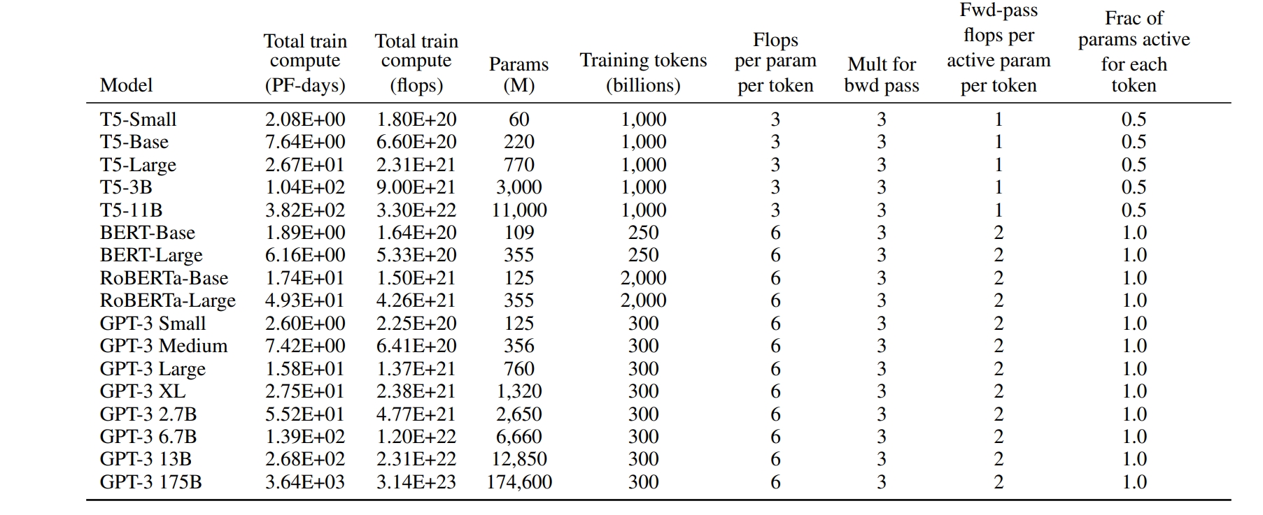
Large Language Model's Costs (https://arxiv.org/pdf/2005.14165v4)
3.6 Training Time Estimation
Given the total FLOPs and the GPU hardware specs, we can estimate training time. The raw GPU FLOP rate alone does not reflect real-world utilization, and typical utilization might be between 0.3 and 0.55 due to factors like data loading, communication, and logging overheads.
Also note that activation recomputation adds an extra forward pass, giving a factor of 4 (forward + backward + recomputation) instead of 3. Thus, per token-parameter we get $2 \times 4 = 8$ FLOPs.
Hence, training time can be roughly estimated by: \(\text{Training Time} \approx \frac{8 \times (\text{tokens count}) \times (\text{model parameter count})} {\text{GPU count} \times \text{GPU peak performance (FLOPs)} \times \text{GPU utilization}}.\)
Example: GPT-3 (175B)
Using 1024 A100 (40GB) GPUs to train GPT-3 on 300B tokens:
- Peak performance per A100 (40GB) is about 312 TFLOPS.
- Assume GPU utilization at 0.45.
- Parameter count $\approx 175\text{B}$.
- Training tokens = 300B.
Estimated training time:
\[\text{Time} \approx \frac{8 \times 300\times 10^9 \times 175\times 10^9} {1024 \times 312\times 10^{12} \times 0.45} \;\approx\; 34\,\text{days}.\]This is consistent with reported real-world results in [7].
Example: LLaMA-65B
Using 2048 A100 (80GB) GPUs to train LLaMA-65B on 1.4T tokens:
- Peak performance per A100 (80GB) is about 624 TFLOPS.
- Assume GPU utilization at 0.3.
- Parameter count $\approx 65\text{B}$.
- Training tokens = 1.4T.
Estimated training time:
\[\text{Time} \approx \frac{8 \times 1.4\times 10^{12} \times 65\times 10^9} {2048 \times 624\times 10^{12} \times 0.3} \;\approx\; 21\,\text{days}.\]This also aligns with [4].
In-Class Question 1: What is the training time of using 4096 H100 GPUs to train LLaMA-70B on 300B tokens?
In-Class Question 2: What is the training time of using 1024 H100 GPUs to train LLaMA-70B on 1.4T tokens?
4. Intermediate Activation Analysis
During training, intermediate activations (values generated in the forward pass that are needed for the backward pass) can consume a large portion of memory. These include layer inputs, dropout masks, etc., but exclude model parameters and optimizer states. Although there are small buffers for means and variances in layer normalization, their total size is generally negligible compared to the main tensor dimensions.
Typically, float16 or bfloat16 is used to store activations. We assume 2 bytes per element for these. Dropout masks often use 1 byte per element (or sometimes bit-packing is used in advanced implementations).
Let us analyze the main contributors for each layer.
4.1 Self-Attention Block
Using: \(Q = x\,W_Q,\quad K = x\,W_K,\quad V = x\,W_V,\) \(\text{Attention}(Q,K,V)= \text{softmax}\Bigl(\frac{QK^\mathsf{T}}{\sqrt{h}}\Bigr)\cdot V,\) \(x_{\text{out}} = \text{Attention}(Q,K,V)\,W_O + x,\) we consider:
- Input $x$
- Shape $[b, s, h]$, stored as float16 $\to 2\,b\,s\,h$ bytes.
- Q and K
- Each is $[b, s, h]$ in float16, so $2\,b\,s\,h$ bytes each. Together: $4\,b\,s\,h$ bytes.
- $QK^\mathsf{T}$ (softmax input)
- Shape is $[b, a, s, s]$. Since $a \times \frac{h}{a}=h$, memory cost is $2\,b\,a\,s^2$ bytes.
- Dropout mask for the attention matrix
- Typically uses 1 byte per element, shape $[b, a, s, s]\to b\,a\,s^2$ bytes.
- Softmax output (scores) and $V$
- Score has $2\,b\,a\,s^2$ bytes, $V$ has $2\,b\,s\,h$ bytes.
- Output projection input
- $[b, s, h]$ in float16 $\to 2\,b\,s\,h$ bytes.
- Another dropout mask for the output: $[b, s, h]$ at 1 byte each $\to b\,s\,h$ bytes.
Summing these (grouping terms carefully), the self-attention block activations total around: \(11\,b\,s\,h + 5\,b\,s^2\,a \quad \text{(bytes, counting float16 and dropout masks)}.\)
4.2 MLP Block
For the MLP: \(x = \mathrm{GELU}(x_{\text{out}}\,W_1)\,W_2 + x_{\text{out}},\) the main stored activations are:
- Input to first linear layer: $[b,s,h]$ at float16 $\to 2\,b\,s\,h$ bytes.
- Hidden activation ($[b,s,4h]$) before or after GELU: $2\times 4\,b\,s\,h = 8\,b\,s\,h$ bytes. (One copy typically for the linear output and one for the activation function input/output; actual usage can vary by implementation.)
- Output of second linear layer: $[b,s,h]$ in float16 $\to 2\,b\,s\,h$ bytes.
- Dropout mask: $[b,s,h]$ at 1 byte per element $\to b\,s\,h$ bytes.
Hence, the MLP block’s stored activations sum to about: \(19\,b\,s\,h \quad \text{bytes}.\)
4.3 Layer Normalization
Each layer has two layer norms (one for self-attention, one for MLP), each storing its input in float16. That is: \(2\times (2\,b\,s\,h) = 4\,b\,s\,h \quad \text{bytes}.\)
Thus, per layer, the activation memory is roughly: \((11\,b\,s\,h + 5\,b\,s^2\,a) + 19\,b\,s\,h + 4\,b\,s\,h \;=\; 34\,b\,s\,h + 5\,b\,s^2\,a.\)
An $l$-layer transformer has approximately: \(l \times \bigl(34\,b\,s\,h + 5\,b\,s^2\,a\bigr)\) bytes of intermediate activation memory.
4.4 Comparison with Parameter Memory
Unlike model parameter memory, which is essentially constant with respect to $b$ and $s$, activation memory grows with $b$ and $s$. Reducing batch size $b$ or sequence length $s$ is a common way to mitigate OOM (Out Of Memory) issues. For example:
- GPT-3 (175B parameters, $96$ layers, $h = 12288, a=96$) at sequence length $s=2048$:
- Model parameters: $175\text{B} \times 2\text{ bytes}\approx 350\text{ GB}$ in float16.
- Intermediate activations:
- If $b=1$, about $275$ GB (close to $0.79\times$ parameter memory).
- If $b=64$, about $17.6$ TB ($\approx 50\times$ parameter memory).
- If $b=128$, about $35.3$ TB ($\approx 100\times$ parameter memory).
Thus, activation memory can easily exceed parameter memory, especially at large batch sizes.
4.5 Activation Recomputation
To reduce peak activation memory, activation recomputation (or checkpointing) is often used. The idea is:
- In the forward pass, we do not store all intermediate activations.
- In the backward pass, we recompute them from stored checkpoints (e.g., re-run part of the forward pass) before proceeding with gradient computations.
This trades extra computation for less memory usage and can cut activation memory from $O(l)$ to something smaller like $O(\sqrt{l})$, depending on the strategy. In practice, a common approach is to only store the activations at certain checkpoints (e.g., after each transformer block) and recompute the missing parts in the backward pass.
5. Conclusion
In this class, we explored how to estimate and analyze key aspects of training for large language models:
- Parameter Count
- For a transformer-based LLM, each layer has approximately $12h^2 + 13h$ parameters, plus $Vh$ for the embeddings, leading to a total of
\(l(12h^2+13h)+Vh.\) - When $h$ is large, we often approximate it as $12\,l\,h^2$.
- For a transformer-based LLM, each layer has approximately $12h^2 + 13h$ parameters, plus $Vh$ for the embeddings, leading to a total of
- Memory Usage
- During training, parameters, gradients, and optimizer states typically use about $20\,\Phi$ bytes under mixed precision with AdamW (where $\Phi$ is the total parameter count).
- Intermediate activations can exceed parameter storage, especially with large batch size $b$ and long sequence length $s$. Techniques like activation recomputation help reduce this memory footprint.
- During inference, only parameters (2 bytes each in float16) and the KV cache are major memory consumers.
- FLOP Estimation
- Roughly 2 FLOPs per token-parameter during a forward pass (one multiplication + one addition).
- Training (forward + backward) yields about 6 FLOPs per token-parameter if no recomputation is used, or 8 FLOPs per token-parameter if activation recomputation is used.
By dissecting these components, we gain a clearer picture of why training large language models requires extensive memory and computation, and how various strategies (e.g., activation recomputation, KV cache) are applied to optimize hardware resources. Such understanding is crucial for practitioners to make informed decisions about scaling laws, distributed training setups, and memory-saving techniques.
6. References
- Raffel C, Shazeer N, Roberts A, et al. Exploring the limits of transfer learning with a unified text-to-text transformer. The Journal of Machine Learning Research, 2020, 21(1): 5485-5551.
- Vaswani A, Shazeer N, Parmar N, et al. Attention is all you need. Advances in neural information processing systems, 2017, 30.
- Brown T, Mann B, Ryder N, et al. Language models are few-shot learners. Advances in neural information processing systems, 2020, 33: 1877-1901.
- Touvron H, Lavril T, Izacard G, et al. Llama: Open and efficient foundation language models. arXiv preprint arXiv:2302.13971, 2023.
- Sheng Y, Zheng L, Yuan B, et al. High-throughput generative inference of large language models with a single gpu. arXiv preprint arXiv:2303.06865, 2023.
- Korthikanti V, Casper J, Lym S, et al. Reducing activation recomputation in large transformer models. arXiv preprint arXiv:2205.05198, 2022.
- Narayanan D, Shoeybi M, Casper J, et al. Efficient large-scale language model training on gpu clusters using megatron-lm. Proceedings of the International Conference for High Performance Computing, Networking, Storage and Analysis, 2021: 1-15.
- Smith S, Patwary M, Norick B, et al. Using deepspeed and megatron to train megatron-turing nlg 530b, a large-scale generative language model. arXiv preprint arXiv:2201.11990, 2022.
Lecture 5: Decoder-only Transformer (LLM) vs Vanilla Transformer: A Detailed Comparison
Introduction
Modern Large Language Models (LLMs) are primarily based on decoder-only transformer architectures, while the original transformer model (“vanilla transformer”) uses an encoder-decoder structure. This class will explore the differences between these two architectures in detail, including their respective advantages, disadvantages, and application scenarios.
Vanilla Transformer Architecture
In 2017, Vaswani et al. introduced the original transformer architecture in their paper “Attention is All You Need.”
Key Features
- Dual-module Design: Consists of both encoder and decoder components
- Encoder:
- Processes the input sequence
- Composed of multiple layers of self-attention and feed-forward networks
- Each token can attend to all other tokens in the sequence
- Decoder:
- Generates the output sequence
- Contains self-attention layers, encoder-decoder attention layers, and feed-forward networks
- Uses masked attention to ensure predictions only depend on already generated tokens
Workflow
- Encoder receives and processes the complete input sequence
- Decoder generates output tokens one by one
- When generating each token, the decoder accesses the complete representation from the encoder through cross-attention
Application Scenarios
Mainly used for sequence-to-sequence (seq2seq) tasks, such as:
- Machine translation
- Text summarization
- Dialogue systems
Decoder-only Transformer (LLM) Architecture
Modern LLMs like the GPT (Generative Pre-trained Transformer) series adopt a simplified decoder-only architecture.
Key Features
- Single-module Design: Only retains the decoder part of the transformer (but removes the cross-attention layer)
- Autoregressive Generation: Predicts the next token based on previous tokens
- Masked Self-attention: Ensures each position can only attend to positions before it
- Scale Expansion: Parameter count is typically much larger than vanilla transformers
Workflow
- The model receives a partial sequence as input (prompt)
- Using an autoregressive approach, it predicts and generates subsequent tokens one by one
- Each newly generated token is added to the input for predicting the next token
Advantages
- Simplified Architecture: Removing the encoder simplifies the design
- Unified Framework: Views all NLP tasks as text completion problems
- Long-text Generation: Particularly suitable for open-ended generation tasks
- Scalability: Proven to scale to hundreds of billions of parameters
Key Differences Comparison
| Feature | Vanilla Transformer | Decoder-only Transformer |
|---|---|---|
| Architecture | Encoder-Decoder | Decoder only |
| Attention Mechanism | Encoder: Bidirectional attention Decoder: Unidirectional masked attention + cross-attention |
Only unidirectional masked self-attention |
| Information Processing | Encoder encodes the entire input Decoder can access complete encoded information |
Can only access previously generated tokens |
| Task Adaptability | Better for explicit transformation tasks | Better for open-ended generation tasks |
| Inference Process | Input processed at once, then output generated step by step | Autoregressive generation, each step depends on previously generated content |
| Parameter Efficiency | Higher for specific tasks | Requires more parameters to achieve similar performance |
| Main Representatives | BERT (encoder-only), T5, BART | GPT series, LLaMA, Claude |
Technical Details
Positional Encoding
Both architectures use positional encoding, but implementation differs:
- Vanilla: Uses fixed sine and cosine functions
- Modern LLMs: Typically use learnable positional encodings or Rotary Position Embedding (RoPE)
Pre-training Methods
- Vanilla (BERT): Masked Language Modeling (MLM) and Next Sentence Prediction (NSP)
- Decoder-only: Autoregressive language modeling, predicting the next token
Attention Mechanism
// Bidirectional self-attention calculation in Vanilla transformer (simplified)
Q = X * Wq
K = X * Wk
V = X * Wv
Attention(Q, K, V) = softmax(QK^T / sqrt(d_k)) * V

// Masked self-attention in Decoder-only transformer
// The main difference is using a mask matrix to ensure position i can only attend to positions 0 to i
mask = generateCausalMask(seq_length)  // lower triangular matrix
Attention(Q, K, V) = softmax((QK^T / sqrt(d_k)) + mask) * V
Why Decoder-only Models Became Mainstream?
- Simplicity: Removes complex encoder-decoder interactions
- Unified Interface: Can transform various NLP tasks into the same format
- Scalability: Proven to scale effectively to massive sizes
- Generalization Ability: Achieves remarkable generalization through large-scale pre-training
Conclusion
While the vanilla transformer architecture excels in specific tasks, the decoder-only architecture has become the preferred choice for modern LLMs due to its simplicity, scalability, and flexibility. Understanding the differences between these architectures is crucial for comprehending current developments in the NLP field.
Each has its advantages, and the choice of architecture should be based on specific task requirements:
- For tasks requiring bidirectional understanding and explicit transformation: Consider vanilla transformers or encoder-only models
- For open-ended generation and general AI capabilities: Decoder-only LLMs are more suitable
Artificial intelligence is developing rapidly, and these architectures continue to evolve, but understanding the fundamental differences will help grasp future development directions.
Lecture 6: Efficient Text Generation of Decoder-Only Transformers: KV-Cache
1. KV Cache
For faster generative inference, transformers often use a KV cache, which stores keys and values from previous tokens so that each new token only attends to the previously computed K and V rather than recomputing them from scratch.
Inference Without KV Cache
During the generation process without KV Cache, each new token is produced as follows:
Initial Token:
Start with the initial token (e.g., a start-of-sequence token). Compute its Q, K, and V vectors, and apply the attention mechanism to generate the first output token.
Subsequent Tokens:
For each new token, recompute the Q, K, and V vectors for the entire sequence (including all previous tokens), and apply the attention mechanism to generate the next token. This approach leads to redundant computations, as the K and V vectors for previously processed tokens are recalculated at each step, resulting in increased computational load and latency.
Inference With KV Cache
The KV Cache technique addresses the inefficiencies of the above method by storing the Key and Value vectors of previously processed tokens:
Initial Token:
Compute the Q, K, and V vectors for the initial token and store the K and V vectors in the cache.
Subsequent Tokens:
For each new token, compute its Q, K, and V vectors. Instead of recomputing K and V for all previous tokens, retrieve them from the cache. Apply the attention mechanism using the current Q vector and the cached K and V vectors to generate the next token. By caching the K and V vectors, the model avoids redundant computations, leading to faster inference times.
With KV Cache, A typical inference process has two phases:
- Prefill Phase: The full prompt sequence ($s$ tokens) is fed into the model, generating the key and value cache for each layer.
- Decoding Phase: Tokens are generated one by one (or in small batches), each time updating and using the cached keys and values.
1.1 Memory Usage of the KV Cache
Suppose the input sequence length is $s$, and we want to generate $n$ tokens. Let $b$ be the inference batch size (number of parallel sequences). We store $K, V \in \mathbb{R}^{b \times (s+n) \times h}$ in float16. Each element is 2 bytes, and we have both $K$ and $V$, so the memory cost per layer is:
\[2 \;\text{(for K and V)} \;\times\; b(s+n)h \;\times\; 2\,\text{bytes} = 4\,b\,(s+n)\,h.\]For $l$ layers, the total KV cache memory is: \(4\,l\,b\,h\,(s+n).\)
GPT-3 Example
Recall GPT-3 has around 350 GB of parameters (in float16). Suppose we do inference with batch size $b=64$, prompt length $s=512$, and we generate $n=32$ tokens:
- Model parameters: 350 GB
- KV cache:
\(4\,l\,b\,h\,(s+n)\approx 164\,\text{GB}\) which is nearly half the parameter size under these settings.
2. Conclusion
In this class, we explored how to estimate and analyze key aspects of inference for large language models:
- A powerful mechanism for fast autoregressive decoding, storing keys and values for each token in float16 to avoid recomputing them.
- The total KV cache scales with $b(s+n)h$ per layer.
By dissecting these components, we gain a clearer picture of why training large language models requires extensive memory and computation, and how various strategies (e.g., activation recomputation, KV cache) are applied to optimize hardware resources. Such understanding is crucial for practitioners to make informed decisions about scaling laws, distributed training setups, and memory-saving techniques.
Lecture 7: Decoding Algorithms in Large Language Models (LLMs)
Decoding algorithms are pivotal in determining how Large Language Models (LLMs) generate text sequences. These methods influence the coherence, diversity, and overall quality of the output. This tutorial delves into various decoding strategies, elucidating their mechanisms and applications.
1. Introduction to Decoding in LLMs
Decoding in LLMs refers to the process of generating text based on the model’s learned probabilities. Given a context or prompt, the model predicts subsequent tokens to construct coherent and contextually relevant text. The choice of decoding strategy significantly impacts the nature of the generated content.
2. Common Decoding Strategies
2.1 Greedy Search
Greedy Search selects the token with the highest probability at each step, aiming for immediate optimality.
Mechanism:
- Step 1: Start with an initial prompt.
- Step 2: At each position $t$, choose the token $x_t$ that maximizes the conditional probability $P(x_t \mid x_{1:t-1})$.
- Step 3: Append $x_t$ to the sequence.
- Step 4: Repeat until a stopping criterion is met (e.g., end-of-sequence token).
Example:
-
Prompt: “The quick brown fox”
- Step 1 (t=1):
Model predicts:- “jumps” (0.65)
- “runs” (0.20)
- “sleeps” (0.15)
→ Greedy selects “jumps”
Sequence: “The quick brown fox jumps”
- Step 2 (t=2):
Model predicts:- “over” (0.70)
- “under” (0.20)
- “beside” (0.10)
→ Greedy selects “over”
Sequence: “The quick brown fox jumps over”
- Step 3 (t=3):
Model predicts:- “the” (0.80)
- “a” (0.15)
- “that” (0.05)
→ Greedy selects “the”
Sequence: “The quick brown fox jumps over the”
- Step 4 (t=4):
Model predicts:- “lazy” (0.60)
- “sleepy” (0.25)
- “hungry” (0.15)
→ Greedy selects “lazy”
Sequence: “The quick brown fox jumps over the lazy”
- Step 5 (t=5):
Model predicts:- “dog” (0.85)
- ”.” (0.10)
- “cat” (0.05)
→ Greedy selects “dog”
Sequence: “The quick brown fox jumps over the lazy dog”
- Stopping Criterion:
The next highest-probability token is the end-of-sequence marker, so generation stops.
- Step 1 (t=1):
Advantages:
- Simple and computationally efficient.
Disadvantages:
- May produce repetitive or generic text.
- Lacks diversity and can miss alternative plausible continuations.
2.2 Beam Search
Beam Search maintains multiple candidate sequences (beams) simultaneously, balancing exploration and exploitation.
Mechanism:
- Step 1: Initialize with the prompt, creating the initial beam.
- Step 2: At each step $t$, expand each beam by all possible next tokens.
- Step 3: Score each expanded sequence using a scoring function, often the sum of log probabilities.
- Step 4: Retain the top $B$ beams based on scores, where $B$ is the beam width.
- Step 5: Repeat until beams reach a stopping criterion.
Example:
Here’s a concrete English example of Beam Search (beam width = 2) generating the sentence “The cat sat on the mat.” Step by step, showing the beam prefixes (what’s in cache), candidate next-tokens with their log-probs, and which beams survive at each iteration.
Prompt (initial beam)
“The cat”
Step 1 (t=1)
We expand “The cat” to all candidate next tokens; here we show the top 4 by log-prob:
| Beam Prefix | Next Token | Log Prob | Cumulative Score |
|---|---|---|---|
| “The cat” | sat | –0.10 | –0.10 |
| “The cat” | is | –1.20 | –1.20 |
| “The cat” | on | –1.50 | –1.50 |
| “The cat” | meows | –2.00 | –2.00 |
Keep top 2 beams (smallest negative score):
- “The cat sat” (–0.10)
- “The cat is” (–1.20)
Step 2 (t=2)
Expand each surviving beam:
| Beam Prefix | Next Token | Log Prob | Cumulative Score |
|---|---|---|---|
| “The cat sat” | on | –0.05 | –0.15 |
| “The cat sat” | quietly | –1.00 | –1.10 |
| “The cat is” | sleeping | –0.20 | –1.40 |
| “The cat is” | hungry | –0.50 | –1.70 |
Keep top 2 beams:
- “The cat sat on” (–0.15)
- “The cat sat quietly” (–1.10)
Step 3 (t=3)
| Beam Prefix | Next Token | Log Prob | Cumulative Score |
|---|---|---|---|
| “The cat sat on” | the | –0.02 | –0.17 |
| “The cat sat on” | a | –0.30 | –0.45 |
| “The cat sat quietly” | on | –0.40 | –1.50 |
| “The cat sat quietly” | in | –0.60 | –1.70 |
Keep top 2 beams:
- “The cat sat on the” (–0.17)
- “The cat sat on a” (–0.45)
Step 4 (t=4)
| Beam Prefix | Next Token | Log Prob | Cumulative Score |
|---|---|---|---|
| “The cat sat on the” | mat | –0.01 | –0.18 |
| “The cat sat on the” | rug | –1.00 | –1.17 |
| “The cat sat on a” | chair | –0.50 | –0.95 |
| “The cat sat on a” | bed | –0.80 | –1.25 |
Keep top 2 beams:
- “The cat sat on the mat” (–0.18)
- “The cat sat on a chair” (–0.95)
Step 5 (t=5)
We stop beams when they output a period token “.”. Only the first beam has that option with a high score:
| Beam Prefix | Next Token | Log Prob | Cumulative Score |
|---|---|---|---|
| “The cat sat on the mat” | . | –0.01 | –0.19 |
| “The cat sat on a chair” | . | –0.05 | –1.00 |
Keep top 1 completed beam:
- “The cat sat on the mat.” (–0.19)
Final Output
The cat sat on the mat.
This illustrates how Beam Search maintains multiple prefixes, scores them, and finally selects the highest-scoring complete sentence.
Advantages:
- Explores multiple hypotheses, reducing the risk of suboptimal sequences.
Disadvantages:
- Computationally more intensive than Greedy Search.
- Can still produce repetitive outputs if not combined with other techniques.
2.3 Sampling-Based Methods
Sampling introduces randomness into the generation process, allowing for more diverse outputs.
2.3.1 Random Sampling
Tokens are selected randomly based on their conditional probabilities.
Mechanism:
- Step 1: Compute the probability distribution over the vocabulary for the next token.
- Step 2: Sample a token from this distribution.
- Step 3: Append the sampled token to the sequence.
- Step 4: Repeat until a stopping criterion is met.
Example:
Given the prompt “Once upon a time”, the model might generate various continuations like “a princess lived” or “a dragon roamed”, depending on the sampling.
Advantages:
- Produces varied and creative outputs.
Disadvantages:
- Can lead to incoherent or less relevant text.
- Quality depends heavily on the underlying probability distribution.
2.3.2 Top-k Sampling
Limits the sampling pool to the top $k$ tokens with the highest probabilities.
Mechanism:
- Step 1: Compute the probability distribution for the next token.
- Step 2: Select the top $k$ tokens with the highest probabilities.
- Step 3: Normalize the probabilities of these $k$ tokens.
- Step 4: Sample a token from this restricted distribution.
- Step 5: Append the sampled token to the sequence.
- Step 6: Repeat until a stopping criterion is met.
Example:
With ( k = 50 ), the model considers only the top 50 probable tokens at each step, introducing controlled randomness.
Advantages:
- Balances diversity and coherence.
- Reduces the chance of selecting low-probability, irrelevant tokens.
Disadvantages:
- The choice of $k$ is crucial; too high or too low can affect output quality.
2.3.3 Top-p (Nucleus) Sampling
Considers the smallest set of top tokens whose cumulative probability exceeds a threshold ( p ).
Mechanism:
- Step 1: Compute the probability distribution for the next token.
- Step 2: Sort tokens by probability in descending order.
- Step 3: Select the smallest set of tokens whose cumulative probability is at least ( p ).
- Step 4: Normalize the probabilities of these tokens.
- Step 5: Sample a token from this distribution.
- Step 6: Append the sampled token to the sequence.
- Step 7: Repeat until a stopping criterion is met.
Example:
With $p = 0.9$, the model dynamically adjusts the number of tokens considered at each step, ensuring that 90% of the probability mass is covered.
Advantages:
- Adapts the sampling pool size based on the distribution, providing flexibility.
- Often results in more natural and coherent text.
Disadvantages:
- Requires careful tuning of $p$ to balance diversity and coherence.
2.4 Temperature Scaling
Temperature scaling adjusts the sharpness of the probability distribution before sampling.
Mechanism:
- Step 1: Compute the logits (unnormalized probabilities) for the next token.
- Step 2: Divide the logits by the temperature $T$ (a positive scalar).
- Step 3: Apply the softmax function to obtain the adjusted probabilities.
- Step 4: Sample a token from this adjusted distribution.
- Step 5: Append the sampled token to the sequence.
- Step 6: Repeat until a stopping criterion is met.
Example:
- With $T = 1$, the distribution remains unchanged.
- With $T < 1$, the distribution becomes sharper, making high-probability tokens more likely.
- With $T > 1$, the distribution flattens, allowing for more diverse token selection.
Advantages:
- Provides control over the randomness of the output.
- Can be combined with other decoding strategies to fine-tune generation behavior.
Disadvantages:
- Setting $T$ too high can lead to incoherent text; too low can make the output deterministic.
In-class Question: Even setting the temperature value as 0, sometimes we can see LLMs to output different outputs given the same prefix. What is the possible cause? Should the LLMs’ outputs always be consistent given the temperature as 0?
Lecture 7: Recent Advances in Large Language Models: Reasoning, Agents, and Vision-Language Models
Introduction
Large Language Models (LLMs) have rapidly progressed from mere text predictors to versatile AI systems capable of complex reasoning, tool use, and multi-modal understanding. This presentation explores three major recent directions in LLM development:
- Reasoning LLMs – techniques that enable step-by-step logical problem solving.
- Autonomous/Tool-Using Agents – letting LLMs use external tools or act autonomously to complete tasks.
- Vision-Language Models (VLMs) – combining visual processing with language understanding.
Each section delves into core concepts, examples (with inputs, intermediate reasoning, and outputs), comparative analyses, and notable research (papers & benchmarks like GSM8K, ARC, Toolformer, ReAct, MM1, GPT-4V). The goal is a deep conceptual understanding of how these advances make LLMs more powerful and general. We include tables, pseudocode, and illustrative figures (with placeholders) to clarify key ideas for a graduate-level audience familiar with transformer models and chat-based LLMs.
1. Reasoning in LLMs: From Answers to Chain-of-Thought
Modern LLMs can do more than recite memorized facts – they can reason through complex tasks. Reasoning LLMs explicitly break down problems into intermediate steps before giving a final answer. This approach addresses the limitation of “one-shot” answering, especially for math, logic, or multi-step questions that standard LLM outputs often get wrong due to missing reasoning steps.
1.1 What Are “Reasoning LLMs”?
A reasoning-enabled LLM is prompted or trained to think step-by-step, mimicking a human’s scratch work or internal monologue. Instead of producing an answer immediately, the model generates a chain of thought (CoT): a sequence of intermediate reasoning steps that lead to the solution (Chain-of-Thought Prompting) (Chain-of-Thought Prompting). These steps can be thought of as the model’s “intermediate scratchpad” where it works through the problem before concluding. By making reasoning explicit, we get two benefits:
- Better Accuracy on complex problems (the model is less likely to skip logic).
- Interpretability, as we can inspect the reasoning the model followed.
Chain-of-Thought Prompting: Introduced by Wei et al. (2022), CoT prompting involves giving the model examples where the reasoning process is written out. This cues the model to follow suit (Chain-of-Thought Prompting) (Chain-of-Thought Prompting). Even without further training, simply adding “Let’s think step by step” or showing worked solutions in the prompt can elicit multi-step reasoning from a sufficiently large model.
Example – Direct vs. Chain-of-Thought:
Consider a math word problem:
Question: “If Alice has 5 apples and buys 7 more, then gives 3 to Bob, how many apples does Alice have?”
-
Standard LLM (direct answer): “Alice has 9 apples.” (The model might do this in one step mentally: 5+7–3 = 9.)
-
LLM with Chain-of-Thought:
Thought 1: “Alice starts with 5 apples and buys 7, so now she has 5+7 = 12.”
Thought 2: “She then gives away 3, so 12–3 = 9.”
Answer: “$\displaystyle 9$.”
Here the chain-of-thought makes the calculation explicit. For simple arithmetic both approaches got it right, but on harder problems the direct method often fails whereas the CoT method succeeds by breaking the task into subtasks.
1.2 Why Chain-of-Thought Helps
Reasoning in steps allows the model to tackle multi-step logic, arithmetic, or commonsense increments rather than leaping to an answer. This significantly improves performance on challenging benchmarks:
- GSM8K (Grade School Math) – a dataset of math word problems. Prompting a 540B model (PaLM) with CoT boosted solve accuracy from 17.9% (standard) to 58.1% – a state-of-the-art result at the time (A Comprehensive Guide to Chain-of-Thought Prompting - Future Skills Academy). In other words, with CoT the model solved over 3× more problems correctly than with a direct approach.
- ARC-Challenge (AI2 Reasoning Challenge) – a hard science question dataset. CoT and related strategies greatly improved performance on this and similar logic benchmarks, approaching or surpassing average human scores as model size grew. (For instance, GPT-4 scored around the 80% range on ARC, nearing human-level, thanks in part to enhanced reasoning ability.)
- Other tasks like MATH (math competition problems), CSQA (commonsense QA), and symbolic reasoning puzzles also saw substantial gains (Chain-of-Thought Prompting) (Chain-of-Thought Prompting). The table below shows how CoT prompting dramatically boosts accuracy across various tasks for a large model:
| Benchmark Task | Standard Prompt Accuracy | CoT Prompt Accuracy | Improvement |
|---|---|---|---|
| GSM8K (Math word problems) | 17.9% (A Comprehensive Guide to Chain-of-Thought Prompting - Future Skills Academy) (PaLM 540B) | 58.1% (A Comprehensive Guide to Chain-of-Thought Prompting - Future Skills Academy) (PaLM 540B) | +40.2% |
| ARC-Challenge (Science QA) | ~70% (GPT-3.5) | ~80% (GPT-4 w/ CoT) | +10% (approx.) |
| MATH (Competition problems) | low (GPT-3) | high (GPT-4 + CoT) | big increase (GPT-4 solves many problems) |
| Commonsense QA (CSQA) | 76% (PaLM) (Chain-of-Thought Prompting) | 80% (PaLM + CoT) (Chain-of-Thought Prompting) | +4% |
| Symbolic Reasoning | ~60% (PaLM) (Chain-of-Thought Prompting) | ~95% (PaLM + CoT) (Chain-of-Thought Prompting) | +35% |
Table: Effect of Chain-of-Thought (CoT) Reasoning on Performance. CoT prompts substantially improve accuracy, especially for complex tasks, when used with large models (100B+ parameters) (Chain-of-Thought Prompting). Smaller models (<10B) often cannot follow CoT correctly, but big models leverage it to reason effectively (Chain-of-Thought Prompting).
The improvements show that prompting the model to “think out loud” mitigates errors from trying to do too much in one step. It also reduces hallucination in reasoning since each step can be checked against the problem.
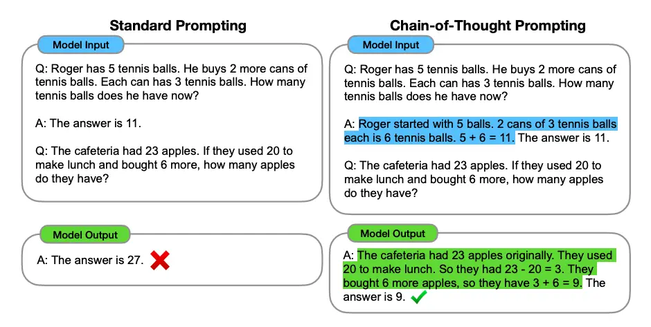
Chain-of-Thought vs Standard Prompting
Illustration: Step-by-step CoT vs. direct answer. The left side shows a naive single-step answer (often incorrect for hard problems), while the right side depicts an LLM enumerating reasoning steps, leading to a correct, justified answer. (By writing out the logic, the model reaches the correct conclusion more reliably.)
1.3 Advanced Reasoning Techniques
Few-Shot vs. Zero-Shot CoT: The initial CoT work used few-shot prompting (providing example solutions). Later, a Zero-Shot CoT method was found: simply appending a trigger phrase like “Let’s think step by step” to the user’s question often induces the model to produce a chain-of-thought even without explicit examples. This works surprisingly well for GPT-3.5/4 class models on many tasks, essentially telling the model to employ CoT reasoning on the fly.
Self-Consistency: One challenge with CoT is that the generated reasoning might occasionally go astray. Self-consistency (Wang et al. 2022) is a technique where the LLM is prompted to generate multiple independent chains-of-thought and answers, then the final answer is chosen by a majority vote or confidence measure across these attempts. This reduces the chance of accepting a flawed single chain-of-thought. It leverages the idea that while any one chain might have an error, the most common answer across many reasoning paths is likely correct. This yielded further performance boosts on GSM8K and other benchmarks beyond a single CoT run.
Tools and External Checks: (Transitioning to next section) Even with step-by-step reasoning, LLMs can struggle with tasks like exact arithmetic or up-to-date factual questions. An emerging idea is to let the model call external tools during its reasoning (e.g. a calculator for arithmetic, or a search engine for facts). This blurs into the territory of LLM agents (Section 2). For example, a reasoning LLM might decide “I should use a calculator for this step” to avoid arithmetic mistakes. This combination of internal reasoning and external tool use is at the frontier of LLM reasoning research (e.g., the ReAct framework discussed soon).
Beyond Linear Chains – Tree-of-Thought: Recent research explores letting the model consider a tree of possible reasoning steps (branching out different approaches) and then search or evaluate the best branch (analogous to game tree search). This “Tree-of-Thought” approach is experimental but aims to handle especially tricky problems by not committing to one line of thought too early. It’s like brainstorming multiple solution paths and then converging on the most promising one. Early results show it can solve some problems that linear CoT cannot, by recovering from false starts on a different branch.
1.4 Example: Chain-of-Thought in Action
Let’s walk through a concrete example demonstrating chain-of-thought reasoning on a more complex question. Consider a typical GSM8K problem:
Question: “Jenny’s age is twice Michael’s age. Five years ago, Jenny was three times as old as Michael. How old is Jenny now?”
A standard LLM might confuse the relations or make a guess. A reasoning LLM will break it down:
- Let’s think step by step. We have Jenny’s age = 2 × Michael’s age (currently). Let J and M be their current ages.
- Equation 1: $J = 2M$.
- Five years ago, Jenny’s age was $J - 5$, Michael’s was $M - 5$.
- At that time, “Jenny was three times as old as Michael” gives Equation 2: $J - 5 = 3(M - 5)$.
- Substitute $J = 2M$ into Eq2: $2M - 5 = 3(M - 5)$.
- Solve: $2M - 5 = 3M - 15$ $\implies$ bring terms: $-5 + 15 = 3M - 2M$ $\implies$ $10 = M$.
- So Michael is 10, and $J = 2M = 20$.
- Answer: Jenny is 20 years old.
Output (LLM): “Jenny is 20 years old.”
Here the model essentially did algebra by writing down the equations in English. Each step follows logically, and even a reader can follow how it reached the answer. This is the power of chain-of-thought prompting – the LLM not only gets the answer right, but shows the reasoning clearly.
1.5 Reasoning LLMs vs. Standard LLMs
To summarize this section, we compare a vanilla LLM (treating it as a black box that directly maps input to output) and a reasoning-enabled LLM:
| Aspect | Standard LLM (direct prompt) | Reasoning LLM (CoT or similar) |
|---|---|---|
| Approach to questions | Answers in one step by next-word prediction – no explicit intermediate output. | Generates a chain of intermediate steps (“thoughts”) before final answer. |
| Interpretability | Low – the reasoning is internal and not visible. | High – the model’s thought process is shown step-by-step, aiding transparency. |
| Performance on complex tasks | Struggles with multi-step problems (math word problems, logical puzzles). Tends to make leaps or mistakes. | Excels at multi-step and logical tasks by tackling them stepwise (A Comprehensive Guide to Chain-of-Thought Prompting - Future Skills Academy). Achieves higher accuracy on benchmarks (GSM8K, ARC, etc.) with CoT prompting. |
| Error characteristics | More likely to hallucinate reasoning or make arithmetic errors silently. | Can still make errors, but easier to spot mistakes in the chain. Allows techniques like self-consistency or manual review to correct steps. |
| Model size needed | Small models can answer factoid questions, but fail at complex reasoning. | CoT is most effective on large models (100B+ params) (Chain-of-Thought Prompting) which have the capacity to follow logical prompts. Smaller models often produce incoherent chains. |
| Example | Q: “What is 37×49?” → “1800” (hallucinated guess, no working shown) | Q: “What is 37×49?” → Thought: “37×50 =1850, subtract 37: 1850–37=1813.” Answer: “1813.” (shows calculation) |
In summary, enabling reasoning in LLMs via prompting or training is a major advancement that has made LLMs far more capable problem solvers. It laid the groundwork for further enhancements – including the ability to use external tools when reasoning, which we discuss next.
2. Autonomous and Tool-Using Agents
While chain-of-thought lets an LLM reason internally, another leap is allowing LLMs to take actions in the world. An LLM agent can interact with external tools or environments (e.g. calling APIs, doing web searches, running code) in a loop of reasoning and acting. This makes LLMs autonomous to a degree – they can be given a goal and then figure out how to fulfill it by themselves, using tools along the way.
Why is this needed? Because even the best purely textual LLM has limitations: it has a fixed knowledge cutoff, it isn’t good at precise calculation or real-time data, and it cannot directly make changes in the world (like sending an email or executing code) just by outputting text. Tool use and autonomy address these gaps:
- Tools extend LLM capabilities: e.g. a calculator for math, a search engine for up-to-date info, a database or code interpreter, etc.
- Autonomy (multi-step planning) allows the model to break a complex goal into sub-tasks, pursue each sub-task (possibly with tools), and adjust if needed – rather than relying on a human to prompt for every intermediate step.
2.1 LLMs as Agents: What Does It Mean?
An LLM agent typically follows a loop: (Observe environment ⇒ Reason ⇒ Act ⇒ Observe new info ⇒ …) until a task is done. The “environment” could be tools like web search or even a simulated world. Unlike a single-turn Q&A, the LLM agent engages in an interactive process.
Key Components of LLM Agents:
- Observation: the agent sees the current state (e.g. user query, or results from last action).
- Reasoning (Thought): the LLM decides what to do next. This is often captured as a textual thought (e.g. “I should look up who this person is.”).
- Action: the LLM outputs an action command instead of a final answer. For example, it might output something like
Search["Apple Remote original program"]. The system executing the agent sees this and performs the action (calls a search API). - Observation (Result): The result of the action (search results text) is fed back to the LLM.
- The cycle repeats: the LLM incorporates the new information, reasons again, possibly takes another action, and so on. Eventually, it outputs a final answer or solution when done.
This architecture lets the LLM branch out of its own internal knowledge and use external information or capabilities as needed.
2.2 Tool Use: From Plugins to Toolformer
OpenAI’s ChatGPT introduced plugins in 2023 which essentially turn it into an agent: the model can decide to call a plugin (tool) like a web browser, calculator, or booking service. “One of the newest and most underrated upgrades to ChatGPT is the plugin feature – the LLM can now decide on its own to use tools to perform actions outside of simple text responses, like booking a flight or fact-checking itself” ( Toolformer: Giving Large Language Models… Tools | by Boris Meinardus | Medium). This was a big practical leap: suddenly LLMs could retrieve real up-to-date information, do computations, or interact with third-party services.
Toolformer (2023) – a research project by Meta – took this idea further by training the model itself to insert API calls into its generation ([2302.04761] Toolformer: Language Models Can Teach Themselves to Use Tools). The model was taught (in a self-supervised way) to decide when a tool could help and to output a call like [Calculator(432 * 19) -> 8208] mid-sentence, get the result, and use it in the continuation. Remarkably, Toolformer (based on a 6.7B model) achieved substantially improved zero-shot performance on various tasks by using tools, often matching much larger (untuned) models ([2302.04761] Toolformer: Language Models Can Teach Themselves to Use Tools). In other words, a medium-sized LLM with tool-use abilities can out-perform a much bigger LLM that’s stuck with its internal knowledge. Tools give “superpowers” without needing to scale the model as much.
Notable tools for LLMs include:
- Calculator – for arithmetic and math (LLMs often make mistakes in math, so delegating to a calculator yields exact results).
- Search engine / Wikipedia – for up-to-date facts or detailed info on obscure queries.
- Database or QA system – some systems use a vector database to find relevant context (related to Retrieval-Augmented Generation, a separate but related idea).
- Code execution – e.g. Python interpreter: the LLM can write code to compute an answer or simulate something (this approach is used in OpenAI’s “Code Interpreter” tool).
- Translator – an LLM might call an external translation API if needed (though modern LLMs themselves are good at translation).
- Custom APIs – e.g. scheduling a meeting, controlling a robot, etc. The sky’s the limit if the model knows the API.
Toolformer’s Approach: It provided a handful of examples of how to use each API, then let the model practice on unlabeled text, figuring out where an API call would help predict the next token better ([2302.04761] Toolformer: Language Models Can Teach Themselves to Use Tools). Through this, it “taught itself” where using a tool makes sense. For instance, in text about dates it might learn to call a date calculation API instead of guessing the date difference. By fine-tuning on this augmented data, the model learned to seamlessly intermix API calls with natural language.
This was a training-time augmentation. Alternatively, one can do it at inference-time via prompting – that’s where frameworks like ReAct come in.
2.3 ReAct: Reasoning + Acting (in Prompt)
ReAct (Yao et al. 2022) is a framework that combines chain-of-thought reasoning with actions in a single prompting paradigm (ReAct Prompting). Instead of just prompting the model for reasoning steps, we also prompt it with an action format. A ReAct prompt typically includes few-shot examples of an agent solving tasks, with a transcript like:
Thought: I need to find more information about X
Action: Search("X")
Observation: [result of search]
Thought: The result suggests Y...
Action: Lookup("Y detail")
Observation: ...
Thought: Now I have enough info to answer.
Answer: [final answer here]
The model, seeing this format, will generate both “Thought” and “Action” lines. The key is that we interleave them: the model produces a thought (reasoning) which leads to an action, gets new info, reasons further, and so on. ReAct thus synergizes reasoning and acting (ReAct Prompting). The reasoning trace helps the model decide the next action, and the retrieved information informs the subsequent reasoning – a positive feedback loop.
Benefits: ReAct was shown to outperform prior baselines on knowledge-intensive tasks (like open-domain QA) and decision-making tasks. By retrieving relevant facts in the middle of its reasoning, it greatly reduces hallucinations and errors. It also makes the process interpretable and controllable – you can watch the agent’s chain-of-thought and intervene if needed. In fact, “ReAct leads to improved human interpretability and trustworthiness of LLMs” and the best results were achieved when combining ReAct with chain-of-thought prompting – essentially using CoT-style thinking for planning actions, which allows use of both internal knowledge and external information.
Illustration: ReAct agent reasoning and acting. The LLM iteratively generates a Thought (blue) explaining what it will do, then an Action (green) which is executed, then sees an Observation (yellow) from the environment. This loop continues until the LLM produces a final answer. Such prompting lets the model handle complex queries by gathering information as needed, rather than relying only on built-in knowledge.
Example – ReAct in practice:
User query: “Aside from the Apple Remote, what other devices can control the program Apple Remote was originally designed to interact with?” (This is a question requiring multi-hop reasoning: identify what “program Apple Remote was designed to interact with”, then find what other devices can control that program.)
A ReAct-enabled agent might proceed:
- Thought 1: “The question asks: Apple Remote (the device) was originally designed to interact with some program. Which program? And then: what other devices can control that program? I should find the program first.”
- Action 1:
Search("Apple Remote originally designed to interact with") - Observation 1: … search results show: “Apple Remote … originally designed to interact with iTunes” …
- Thought 2: “It’s iTunes. Now the question: what other devices can control iTunes?”
- Action 2:
Search("devices that can control iTunes") - Observation 2: … results: “iTunes can be controlled by Apple Remote, and also by iPhone, iPad via Remote app, etc.”
- Thought 3: “It seems other devices include iPhones, iPads (via the Remote app), and possibly third-party remotes.”
- Answer: “It was designed for iTunes, which can also be controlled by devices like the iPhone or iPad (running the Remote app) in addition to the Apple Remote.”
This illustrates how the agent figured out the answer via two web searches, something a single-turn LLM without tool use might not have known. The thoughts guided the search actions, and the retrieved info was integrated into the reasoning. ReAct prompting enabled this entire chain inside the LLM.
Pseudocode: ReAct Agent Loop (simplified):
state = initial_question
while True:
    output = LLM(prompt_with(state))
    # LLM generates either a Thought, an Action, or Final Answer based on prompt format.
    if output.type == "Action":
        result = execute_tool(output)
        state += "\nObservation: " + result  # add result to the prompt
        continue  # loop back for another thought
    elif output.type == "Answer":
        print("Final Answer:", output.text)
        break
This loop continues until the model emits an answer rather than an action. In prompt engineering terms, the prompt contains the dialogue of thoughts/actions, and each iteration extends it. This is how frameworks like LangChain implement LLM agents using ReAct – by programmatically detecting the “Action:” and feeding back the tool’s result.
2.4 Autonomous Agents: Beyond Single Tools
With the ability to use tools, developers combined it with goal-driven loops to create autonomous agents like AutoGPT and BabyAGI (popular open-source projects in 2023). These tie an LLM to a cycle of:
- Taking a high-level goal (e.g. “Research and write a report on XYZ”),
- Breaking it into sub-tasks,
- Executing tasks (using tools or the LLM itself for each),
- Generating new tasks from results until the goal is completed.
These systems often maintain a task list and a memory, allowing the LLM to keep track of progress. For example, AutoGPT can spawn new “thoughts” like “I should search for information A, then use that to get B, then compose a report.” It then carries out the plan with minimal human intervention, effectively acting like an autonomous agent that iteratively prompts itself.
HuggingGPT (Microsoft, 2023) demonstrated an agent that uses an LLM (ChatGPT) as a controller to orchestrate multiple AI models on Hugging Face for complex tasks (e.g., a multi-step task involving image generation, object detection, and language). The LLM decides which specialized model to call at each step – a form of tool use where tools are other AI models.
Generative Agents (Interactive Sims) (Stanford, 2023) took autonomy in a different direction – they put multiple LLM-based agents in a simulated game environment (like The Sims) to see if they could exhibit believable, emergent behaviors. Each agent could make plans (e.g. “go to the cafe at 3pm to meet a friend”) and remember interactions. This showcases that when given long-term memory and goals, LLM agents can indeed act in an autonomous, adaptive manner over extended periods, not just single Q&A sessions.
2.5 Comparison: Agent vs. Plain LLM Prompting
It’s important to understand how this new agent paradigm contrasts with the classic single-turn prompt usage:
| Characteristic | Plain LLM Prompt | LLM as Agent |
|---|---|---|
| Interaction Style | One-shot or few-shot query → response. No follow-up by the model; any iteration is driven by the user. | Multi-turn loop. The LLM can initiate actions and request information. It’s an interactive dialog between the LLM and tools. |
| Use of External Info | Limited to what’s in model’s training data or provided in prompt. Cannot fetch new data mid-response. | Can call tools/APIs to get fresh info (web search, DB queries, etc.) ( Toolformer: Giving Large Language Models… Tools). Can incorporate real-time data and computation results into its reasoning. |
| Problem Solving | Solves in one step. Struggles with lengthy or decomposed tasks unless user manually breaks it down. | Can decompose tasks itself. Handles more complex goals by planning sub-tasks, executing them sequentially. More autonomous in figuring out what to do next. |
| Memory | Limited to prompt window per turn (though can have some long context, it’s passive). | Can implement long-term memory via storage (e.g., the agent can save notes or update a context that persists across turns). More like a cognitive loop than a one-off response. |
| Transparency | Only final answer is seen (unless model is prompted to explain). Harder to diagnose errors. | Intermediate thoughts and actions are visible (by design in ReAct). Easier to trace how it got to an answer; one can debug which action led to an error. |
| Examples | Q: “What’s the capital of France?” → “Paris.” (No external call, answer from knowledge) | Q: “Who won the Best Actor Oscar in 2020 and give one of their movie quotes.” → Agent might Search for Oscar 2020 Best Actor (finds Joaquin Phoenix), then search for famous quotes by him, then respond with the info. |
In essence, agentic LLMs are more powerful and flexible – they decide how to solve a problem, rather than just solving it in one shot. However, this comes with challenges:
- The agent might get caught in loops or take irrelevant actions if not properly constrained.
- There’s higher complexity in orchestrating the prompt format, tool APIs, and maintaining state.
- Cost can be higher (multiple API calls to the LLM and tools).
- Ensuring safety is trickier: an autonomous agent could potentially do harmful things if instructed maliciously (e.g. use a tool to send spam emails). Safeguards and monitored execution are needed.
2.6 Notable Research and Developments in LLM Agents
- ReAct (2022) – Already discussed; a seminal approach combining reasoning and acting in prompting (ReAct Prompting). It influenced many tool-using agent frameworks (LangChain’s agents are based on ReAct format, for example).
- MRKL (2022) – An earlier concept (Modular Reasoning, Knowledge and Language) that routed an LLM’s queries to different tools or experts. It was a precursor to the idea of an LLM orchestrating tool use.
- Toolformer (2023) – Fine-tuned model that learned tool API usage self-supervised ([2302.04761] Toolformer: Language Models Can Teach Themselves to Use Tools). Showed even relatively small models gain a lot by using tools (often matching much larger models that lack tool-use).
- HuggingGPT (2023) – The LLM as a master controller calling other models for specific tasks (e.g., using a vision model for an image task, a speech model for audio, etc.). It treats each model as a tool and sequences calls to them based on the high-level request.
- AutoGPT/BabyAGI (2023) – Community-driven agent examples that popularized the concept of an “AI agent” that can iteratively improve and work towards open-ended goals. They showed the excitement (and pitfalls) of letting GPT-4 run autonomously (users found they can be creative but sometimes hilariously inept or stuck).
- Self-Refine / Reflexion – Methods where the LLM agent can critique its own outputs or mistakes and try again (essentially giving it a reflective capability to avoid repeating errors).
- Real-world agents: Efforts to use LLM agents in physical domains, like robotics (e.g., an LLM controlling a robot with actions like “pick up the cube” – possibly using a tool API that interfaces with robot controls). Also, agents in simulated environments (game AI, as mentioned with Generative Agents).
The agent paradigm is pushing us toward more interactive AI. Instead of just answering questions, LLMs are starting to function as cognitive engines that can do things: read the web, manipulate files, control other applications, etc. This opens up many possibilities – an AI that can research a topic thoroughly and then write a summary, or an AI that can take a user’s request “Plan my weekend trip” and actually go book hotels, find restaurants (by using tools).
It also raises new research questions on how to ensure these agents remain reliable, safe, and efficient. Combining reasoning with action is a big step toward more general AI behavior.
Key Takeaway: Autonomous and tool-using agents extend LLMs beyond text prediction – they can interact with external systems and iteratively plan, making them far more capable on complex, real-world tasks than static prompts. This is a major frontier in 2024–2025 LLM research and applications. The next section will look at another frontier: extending LLMs to multimodal inputs, especially vision, which further broadens what these models can do.
3. Vision-Language Models (VLMs): Multimodal LLMs
Humans don’t only communicate with text – we perceive the world in images, sounds, etc. A long-standing goal in AI has been to build models that can see and talk: interpret images and describe them, or take visual context into account for reasoning. Vision-Language Models (VLMs) are systems that integrate visual processing with language understanding/generation. Recent advances have effectively combined the power of LLMs with powerful vision models, creating multimodal LLMs that accept images (and sometimes other modalities like audio) as part of their input and produce useful language outputs (captions, answers, explanations, etc.).
Why is this important? Consider tasks like:
- Describing what’s happening in a picture (image captioning).
- Answering a question about an image (Visual QA): e.g. “What is the color of the car in this image?”.
- Explaining a meme or infographic.
- Interpreting a chart or graph and answering questions about it.
- Helping a visually impaired user by understanding an image they send.
- Multimodal reasoning: e.g. “From the plot in this paper, does increasing X appear to increase Y?” – requiring reading a graph and using knowledge.
A pure text model can’t do these, and a pure vision model doesn’t produce rich language. The synergy of VLMs enables such applications.
3.1 How Vision-Language Models Work (Conceptually)
At a high level, a VLM combines a visual encoder (to process images into some representation) with a language model (to turn that representation into text, or to use it in reasoning). There are a few design patterns:
-
Dual Encoder (CLIP-style): One network for images, one for text, trained to produce embeddings that match for the same concept. This was introduced by OpenAI’s CLIP (Contrastive Language–Image Pre-training) in 2021 (CLIP: Connecting text and images). CLIP learned visual concepts from 400M image-text pairs by training such that, say, the embedding of an image of a dog is close to the embedding of the text “a dog”. CLIP itself isn’t a generator, but it’s great at understanding images and mapping them to labels or captions via similarity. It demonstrated zero-shot image classification: provide the names of classes (text) and it will pick which is most similar to the image embedding, effectively classifying without explicit training on those classes. CLIP became a foundation for many later VLMs (it provides a strong vision encoder).
-
Encoder-Decoder (Captioning style): An image encoder produces features which are fed into a language decoder (like a GPT or a Transformer decoder) to generate a caption or answer. This is like the classic image captioning models, but scaled up with transformers. E.g., ViLBERT, VisualBERT (2019) fused image regions and text in a BERT-like model for vision-and-language understanding tasks. Those were early VLMs focused more on understanding than generation.
-
Interleaved multimodal models: These models, like Flamingo (DeepMind, 2022), accept sequences that mix images and text. Flamingo has a vision encoder (like a pre-trained EfficientNet or Vision Transformer) whose outputs are injected into a language model through special cross-attention layers (Flamingo: a Visual Language Model for Few-Shot Learning - arXiv). It can take in a few example image–text pairs followed by a new image, and then generate text for the new image (few-shot learning). “Flamingo… takes as input a prompt consisting of interleaved images, videos, and text and then outputs associated language,” achieving state-of-the-art few-shot learning on a wide range of open-ended multimodal tasks (Tackling multiple tasks with a single visual language model - Google DeepMind). This was a breakthrough – one model handling image+text in a prompted way, similar to how GPT-3 handles just text prompts. It set new SOTA on tasks like image captioning and visual question answering with only a handful of examples given (no task-specific finetuning) (Tackling multiple tasks with a single visual language model - Google DeepMind).
-
Two-Stage Models (BLIP-2 style): An efficient approach used by BLIP-2 (2023) is to keep a frozen image encoder (like CLIP’s or ViT) and a frozen large language model (like GPT-style), and learn a small bridge module in between (the Q-Former). The Q-Former takes the image features and produces a handful of “query embeddings” that summarize the visual info, which are then fed into the LLM’s input embedding space (BLIP-2: Bootstrapping Language-Image Pre-training with Frozen …). This way, the heavy vision and language components don’t need retraining – only the intermediate adapter is trained. BLIP-2 demonstrated you can connect a pre-trained ViT and a pre-trained LLM to get a capable VLM without full retraining. It can do zero-shot VQA and captioning quite well.
-
Multimodal Fine-tuned LLMs: Models like LLaVA, MiniGPT-4, and GPT-4’s vision represent taking an LLM (sometimes a smaller fine-tuned one like Vicuna for MiniGPT-4, or the actual GPT-4 for OpenAI’s product) and feeding images into it via a projection. LLaVA (Large Language and Vision Assistant) in 2023 fine-tuned LLaMA (a language model) with images by mapping image features into the LLM’s embedding space and training on a conversational VQA dataset. The result is a chatbot that can “see” images and respond about them. OpenAI’s GPT-4V (GPT-4 Vision, launched 2023) is the most advanced example – it’s a version of GPT-4 that accepts image inputs in addition to text, and can output detailed answers or descriptions.
Note: Although initial VLM research had separate “vision encoders” and “text decoders”, the trend with GPT-4V and others is to unify them: essentially a giant model with both vision and language capabilities integrated. For instance, GPT-4’s vision component is not fully disclosed, but it likely uses a dedicated vision module whose output is fed into the same transformer as the text (some reports suggest a form of early fusion after the first few transformer layers). Apple’s MM1 (2024) also follows a unified large-scale multimodal model approach, training up to 30B parameter models that handle image+text together ([2403.09611] MM1: Methods, Analysis & Insights from Multimodal LLM Pre-training).
3.2 Capabilities of Modern VLMs
Today’s state-of-the-art VLMs, like GPT-4V and MM1, exhibit impressive capabilities:
- Visual Description and Captioning: They can generate detailed captions for images. E.g., show an image from a city street and the model can produce: “A busy street in New York City with yellow taxis in traffic and people crossing the crosswalk.”
- Visual Question Answering (VQA): You can ask a question about an image. For example, provide a photo and ask “How many people are in this photo and what are they doing?” The model can count the people and describe their activity.
- OCR and Document Understanding: GPT-4V can read text in images (OCR) and interpret it in context. E.g. you can upload a screenshot of a document and ask questions about it. It can also do things like analyze a chart image (bar graph, pie chart) and answer questions about the data.
- Reasoning on images: This is new – models like GPT-4V can do some reasoning that involves visual elements. For instance, explaining a joke in a meme image (which might require recognizing an object and understanding the cultural/contextual humor). One famous example: an image with a convoluted HDMI adapter chain was given to GPT-4 and it was asked “Why is this funny?” GPT-4V correctly explained that the absurdly impractical chain of adapters made it humorous. This kind of high-level reasoning on visual input was essentially unattainable before multimodal LLMs.
- Multi-Image tasks: Apple’s MM1 emphasizes multi-image reasoning, i.e., the model can take multiple images in the context (like frames of a comic or a before/after image) and reason across them ([2403.09611] MM1: Methods, Analysis & Insights from Multimodal LLM Pre-training) (Apple’s MM1. Exploring the frontier of Multimodal). For example, comparing two medical images or tracking changes across time.
- Enhanced few-shot learning: MM1’s research found that training on interleaved image-text data gave their model strong in-context learning abilities with images (like Flamingo had). It can see a couple of examples of a new image task and then do a new one few-shot ([2403.09611] MM1: Methods, Analysis & Insights from Multimodal LLM Pre-training).
Notable Benchmarks:
Vision-language models are evaluated on an array of benchmarks:
- COCO Captions – generating captions for MS COCO images.
- VQAv2 – Visual QA dataset where the model answers open-ended questions about images.
- OK-VQA – VQA requiring outside knowledge (not just what’s in the image, e.g., “What is the name of the monument in the picture?” requires knowing that monument’s name – a blend of vision and world knowledge).
- NoCaps – image captioning with novel objects not seen in training.
- VizWiz – VQA on images taken by blind users (often low-quality images, so a robust understanding needed).
- TextCaps – captioning images that contain text (requires reading the text in the image and incorporating it).
- Science charts/diagrams – e.g., the MathVista and ChartQA benchmarks test if models can interpret scientific plots or math diagrams.
Recent models have achieved impressive results:
- Apple’s MM1-30B outperforms previous models (like Flamingo-80B by DeepMind, and Meta’s IDEFICS-80B) on captioning benchmarks (COCO, NoCaps, TextCaps) and on VizWiz-QA in few-shot settings (Apple’s MM1. Exploring the frontier of Multimodal). This is notable because it’s smaller than those models but better – thanks to a good training recipe. It shows how quickly the field is progressing that a 30B model (with MoE) can beat an 80B from a year prior on several tasks.
- However, the competition is fierce: the same report notes other models like Emu-2 (37B) and LLaVA-Next (34B) were competitive or better on VQAv2 and OK-VQA (Apple’s MM1. Exploring the frontier of Multimodal). So there’s no single model that dominates every task yet; some are better at factual QA, others at fine-grained captioning, etc. This indicates the field is still evolving and models are being specialized or tuned for certain strengths.
- GPT-4V (multimodal GPT-4) hasn’t been officially benchmarked on all academic datasets publicly, but anecdotal and limited evaluations suggest it’s at or near SOTA on many tasks. For example, one study found GPT-4V outperformed other approaches on complex benchmarks like MathVista (diagram reasoning) and ChartQA (chart-based QA) (Assessing GPT4-V on Structured Reasoning Tasks). In VQAv2, early tests showed GPT-4V scored very highly (possibly even exceeding human performance in some settings), but those numbers are yet to be fully confirmed in publications.
Table: Selected Vision-Language Models and Their Features
| Model | Year | Organization | Size | Modalities | Notable Capabilities |
|---|---|---|---|---|---|
| CLIP | 2021 | OpenAI | ~400M (encoders) | Image & Text (dual encoder) | Learned joint image-text embeddings; enabled zero-shot image classification matching ResNet-50 accuracy on ImageNet without using any labeled training images (CLIP: Connecting text and images). Widely used as a vision backbone. |
| Flamingo-80B | 2022 | DeepMind | 80B LLM + vision enc. | Image & Text (interleaved) | First large VLM for few-shot learning. Set SOTA on few-shot VQA, captioning (Tackling multiple tasks with a single visual language model - Google DeepMind). Accepts interleaved image-text prompts (e.g. image, question about it, etc.). |
| PaLI-17B | 2022 | 17B (encoder-decoder) | Image & Text (encoder-decoder) | Trained on multilingual image captions and VQA. Strong on captioning and VQA, handling multiple languages. Demonstrated multi-task learning (unifying vision tasks). | |
| BLIP-2 | 2023 | Salesforce | ~1B (ViT) + 6B (LLM) | Image & Text (two-stage) | Uses a frozen ViT and frozen LLM with a learned Q-Former bridge (BLIP-2: Bootstrapping Language-Image Pre-training with Frozen …). Efficient yet effective zero-shot VQA and captioning. Can plug in different LLMs (e.g. Flan-T5 or GPT-like) for different trade-offs. |
| Kosmos-1 | 2023 | Microsoft | 1.6B | Image & Text (unified) | One of the first attempts at a multimodal GPT-like model. Showed ability on image-based IQ tests and joint vision-language tasks. Pioneered treating images as just another input token sequence in a transformer. |
| LLaVA | 2023 | Community (UC Berkeley/MBZUAI) | 13B (LLaMA) | Image & Text (projected to LLM) | Fine-tuned an open LLM (LLaMA) with image inputs (via CLIP-ViT to LLM projection). Turns LLaMA into a multimodal chatbot that can do VQA and descriptions. Open-source analog of ChatGPT-vision (with lower capability). |
| GPT-4V | 2023 | OpenAI | ~>100B (est.) | Image & Text (unified, multimodal) | GPT-4 with vision input. Outstanding reasoning on images: can interpret memes, diagrams, OCR text, solve visual puzzles. In a casual setting, can describe images or answer complex questions about them. Likely at or near SOTA on many vision-language tasks (OpenAI reported strong results on internal tests). |
| Apple MM1-30B | 2024 | Apple | 30B (with MoE) | Image & Text (unified) | Achieved SOTA on several benchmarks (captioning, VizWiz) outperforming larger models (Apple’s MM1. Exploring the frontier of Multimodal). Supports multi-image inputs and few-shot chain-of-thought reasoning with images ([2403.09611] MM1: Methods, Analysis & Insights from Multimodal LLM Pre-training) (Apple’s MM1. Exploring the frontier of Multimodal). Signals Apple’s entry into large-scale VLMs. |
(Table: A timeline of notable Vision-Language Models, showing the rapid progress in capabilities. Models have grown in sophistication from dual encoders like CLIP to fully integrated multimodal LLMs like GPT-4V and MM1.)
3.3 Examples: Vision-Language Tasks
To ground these concepts, let’s run through a few example scenarios a modern VLM can handle:
Image Captioning Example:
(Input: an image of a family having a picnic under a tree.)
Model output: “A family of four enjoys a picnic on a sunny day. A spread of food is laid out on a blanket under a large tree, while the parents and children smile and interact.”
Intermediate reasoning: The model’s vision module identifies people, a picnic setup, the tree, sunny weather, etc., and the language module weaves it into a coherent sentence. (If we had the chain-of-thought, it might be something like: detects objects → infers scene → produces descriptive sentence.)
Visual Question Answering Example:
(Input: an image of a man standing next to a bicycle on a mountain trail, and the question: “Is the person likely on a leisure activity or working?”)
Model reasoning (imagined): Sees man with bicycle on a scenic trail, likely not in work uniform, context suggests recreation → “He is likely engaged in a leisure activity (biking on a trail for fun).”
Model answer: “It appears to be a leisure activity – he’s biking on a mountain trail for recreation.”
This requires understanding context and common sense from the image.
OCR + Reasoning Example:
(Input: a photo of a sign that reads “Parking $5 per hour, $20 per day”, question: “How much would 3 hours of parking cost?”)
The model must read the text “$5 per hour, $20 per day”, then do math.
Answer: “3 hours would cost $15.”
Analysis: The vision component does OCR (“$5 per hour, $20 per day”), the language/logic part interprets the pricing and calculates 3×$5. This blends vision (reading) with reasoning (simple math).
Multi-image Reasoning Example:
Imagine feeding two images: one of a jar 3/4 full of water, another of the same jar 1/4 full, and asking: “Which photo shows more water and by what difference roughly?”
The model needs to compare images: It can determine the first has more (3/4 vs 1/4, a difference of about half a jar).
Answer: “The first image has significantly more water – roughly half a jar more water than the second image.”
Some advanced models explicitly allow multiple image inputs in a single context (e.g., “Image1: …; Image2: …; Question: …”).
Explaining a Meme (Complex Reasoning) Example:
(Input: an image meme – say a famous “Distracted Boyfriend” meme – with the question: “What is the joke here?”)
The model needs to identify the scene: A guy looking at another woman while his girlfriend is upset. Then recall or recognize this as a meme format about being distracted by something new.
Answer (GPT-4V style): It would explain that the humor comes from the universal scenario of someone being distracted from their partner by someone else – often labeled in memes as e.g. “My study time” (girlfriend) and “a new video game” (the girl being looked at), etc. The model might say: “It’s the ‘Distracted Boyfriend’ meme, showing a man holding hands with his girlfriend but obviously turning to look at another woman. The joke is about being distracted by something more appealing even when you should be paying attention to what you already have, often used metaphorically.”
This is high-level interpretation requiring not just object recognition but understanding the social context and the fact it’s a well-known internet meme format.
These examples show a spectrum from straightforward perception to sophisticated reasoning involving vision + language.
3.4 Challenges and Recent Research in VLMs
Combining vision and language isn’t trivial. Some challenges and active research areas include:
- Aligning the Modalities: Training a model to jointly understand image and text without one dominating or confusing the other. (E.g., early attempts sometimes had the model just ignore the image and rely on priors to answer questions; careful loss balancing is needed to ensure image features are used.)
- Efficiency: Images are high-dimensional. Feeding an entire image as pixels into a transformer with text would be computationally huge. So we use CNN or ViT encoders to compress images first. Even then, handling multiple images or high-res images is heavy. Apple’s MM1 paper found that image resolution and token count significantly impact performance, whereas the exact architecture of the vision-language connector might be less critical ([2403.09611] MM1: Methods, Analysis & Insights from Multimodal LLM Pre-training). They also highlight the cost of multi-image input.
- Visual hallucination: Just like LLMs hallucinate facts, VLMs can hallucinate details not present in the image (e.g., saying “a red car” when the car was blue). Ensuring the model’s output stays grounded in the visual evidence is an ongoing concern. Some approaches to mitigate this include training with grounded learning objectives or using visual prompting (explicitly asking the model to describe what it sees before answering a question, to separate perception from prior knowledge).
- Benchmarks beyond static images: There’s interest in extending to video (temporal reasoning, e.g., describe a video or answer questions about a movie clip) and audio (truly multimodal models like Meta’s ImageBind aim to join image, text, audio, etc. in one space). GPT-4’s current public version doesn’t handle video or audio, but research models are tackling these.
- In-context learning with vision: Flamingo and MM1 show few-shot prompting can work (giving example image-question-answer triples). Others are exploring instruction tuning with multimodal data (like the open InstructBLIP which fine-tuned BLIP-2 on a variety of user instruction data with images).
- Safety and ethics: Vision adds new dimensions to consider, such as not revealing private info from images (face recognition, etc.), avoiding biases (not making problematic assumptions from appearance), and handling potentially graphic or sensitive images appropriately. OpenAI’s GPT-4V, for example, refuses to identify people in images and has filters for certain content. Research continues on making sure these models behave safely with visual input.
Notable recent works and benchmarks:
- MMBench or MMBig: large suites of tasks to evaluate multimodal LLMs on everything from simple captioning to complex reasoning and OCR.
- Vision-augmented CoT (v-CoT): A method where you prompt the model to first describe the image and gather visual facts, then reason – essentially chain-of-thought but including visual descriptions. Early research suggests that prompting GPT-4V in this way can improve performance on tasks like chart reasoning (Assessing GPT4-V on Structured Reasoning Tasks) (Assessing GPT4-V on Structured Reasoning Tasks).
- Multimodal eval of GPT-4V: Some papers evaluate GPT-4V on niche tasks, like understanding scientific diagrams or doing infographics QA. Often GPT-4V does very well, but interestingly one study found on a highly abstract visual reasoning test (Chollet’s ARC with images), GPT-4V did worse than GPT-4 text-only + a human-written description of the image (Assessing GPT4-V on Structured Reasoning Tasks). This indicates that for certain problems, breaking the task into “describe image then use text model” might still be better – an area for future improvement.
3.5 A Unified Future: Multimodal Reasoning and Acting
Having covered reasoning, tools, and vision separately, it’s worth noting that the long-term trend is to combine these advancements. For instance:
- An ideal assistant might take in text and images, think step-by-step, use tools when needed, and produce answers.
- GPT-4 already combines vision and reasoning (we saw it can do CoT on images in research).
- One can integrate tool use in multimodal models as well (e.g., an agent that can see an image and decide to call an OCR API or a specific vision tool – though GPT-4V doesn’t need OCR API since it has it built-in).
- Robotics is a domain where all three converge: say a robot with a camera (vision) using an LLM to plan (reasoning) and act (control robot or query tools). There are research projects like PaLM-E (Google, 2023) which integrated a language model with embodied control, allowing an LLM to process visual observations from a robot and output actions in the form of navigation or manipulation commands.
Apple’s MMXL (hypothetical): If MM1 is extended, perhaps they or others will include audio, spatial data, etc., making multi-multimodal models. The trend is moving from LLM to LLM++ (language + other modalities, plus reasoning and tool interfaces).
Conclusion
Transformer-based LLMs have evolved from pure text predictors to general problem solvers. We examined three cutting-edge dimensions of this evolution:
-
Reasoning LLMs: By leveraging chain-of-thought prompting and related techniques, LLMs can perform complex reasoning tasks previously out of reach, achieving far better results on benchmarks like GSM8K and ARC (A Comprehensive Guide to Chain-of-Thought Prompting - Future Skills Academy). This makes them more reliable and transparent in logical domains.
-
Autonomous/Tool-Using Agents: Giving LLMs the ability to use tools and act in a loop transforms them into interactive agents. They can fetch information, run computations, and perform multi-step workflows on their own, greatly extending their capabilities beyond what’s stored in their parameters ([2302.04761] Toolformer: Language Models Can Teach Themselves to Use Tools). Frameworks like ReAct (ReAct Prompting) demonstrate how reasoning and acting together yield more powerful systems, and projects like AutoGPT hint at the potential (and challenges) of AI agents pursuing open-ended goals.
-
Vision-Language Models: Integrating visual understanding with language allows AI to interpret and describe the world in rich detail. Modern VLMs can caption images, answer visual questions, and even reason about visual content, powered by advances like CLIP’s representations (CLIP: Connecting text and images) and huge multimodal models like GPT-4V. This brings AI closer to human-like perception and understanding, enabling applications from aiding the visually impaired to analyzing scientific figures.
These advancements do not exist in isolation – the most exciting systems combine all three. For example, a medical assistant AI might look at a patient’s X-ray (vision), reason through a diagnosis (CoT), and consult medical databases or calculators (tools) before giving an answer. Each component we discussed adds a layer of capability:
- Reasoning gives depth (the “thinking” skill),
- Agents/Tools give breadth and action (the “doing” skill),
- Vision multimodality gives perception (the “seeing” skill).
Together, they are pushing AI toward more general intelligence – systems that can perceive, think, and act.
The research landscape in 2024-2025 is incredibly active. Notable papers like Toolformer, ReAct, PaLM-E, Flamingo, BLIP-2, GPT-4 Technical Report, MM1, etc., mark the milestones we discussed, and new ones are emerging constantly. Benchmarks continue to get tougher, and models continue to rise to the challenge – often rapidly outpacing prior state-of-the-art within months.
For a graduate student studying these topics, key takeaways are:
- Prompt engineering and clever use of LLMs (like CoT and ReAct) can dramatically improve performance without changing model architecture.
- There is a trend towards interactivity – making LLMs active agents rather than passive answerers.
- Multimodality is breaking the barrier between text and the rest of the world, which will unlock far more applications (and also requires multidisciplinary knowledge of vision, NLP, etc.).
- Scale is not the only path; many of these advances achieve more by using models smarter (e.g., a 6B Toolformer doing what a 175B couldn’t because it lacked tools).
In conclusion, the progress in these three areas – reasoning, agents, and VLMs – represents a significant step change in what AI systems can do. They are more intelligent in a practical sense: they can reason through hard problems, take actions to get information or affect the world, and understand multiple modalities. As research continues, we can expect future LLM-based systems to seamlessly integrate all these abilities, bringing us closer to AI that can see, think, and act in the world much like an human assistant would (albeit with superhuman knowledge and speed in certain aspects). It’s an exciting time, and the lines between “language model” and “general AI agent” are increasingly blurring.
Top 6 students who have great performance in the In-Class Question Answering:
Dalin Annappa, Lavanya
Wu, Jianbo
Du, Shangjie
Amanbayev, Abylay
Qiu, Weimin
Seth, Siddharth
This is to acknowledge the above students’ active participation in this course’s learning about LLMs’ knowledge and their great intelligence on the fast and correct reponses to the in-class questions.